This is my summary of this 2021 paper from the Mizrahi lab.
Figure 1: Imaging in naive mice
The used Tbet-cre to target MC and TCs, and identified them as putative MCs based on their depth.
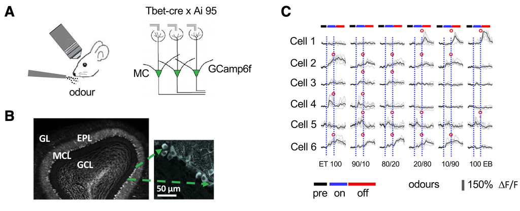
They imaged in naive mice in 10 second bouts per odour: 4 seconds pre, 2 seconds during the odour, and 4 seconds after, followed by an ITI of 5 seconds. Odours (including a blank) were presented in random odour.
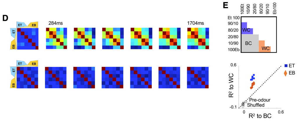
When plotting how similar odour representations were over time, they observed organization by chemical identity:
Individual cells tended to respond with either step-like templates to the odour mixtures, like has been reported before in zebrafish – but also with ramp-like templates.
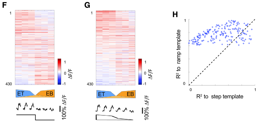
The main message of imaging in these awake mice, passively exposed to odour, is that representations are chemically driven.
Figure 2: Behavioural paradigm
They use a go-no-go task, where mice have to detect a rewarded odour, then likc a water spout to receive reward:
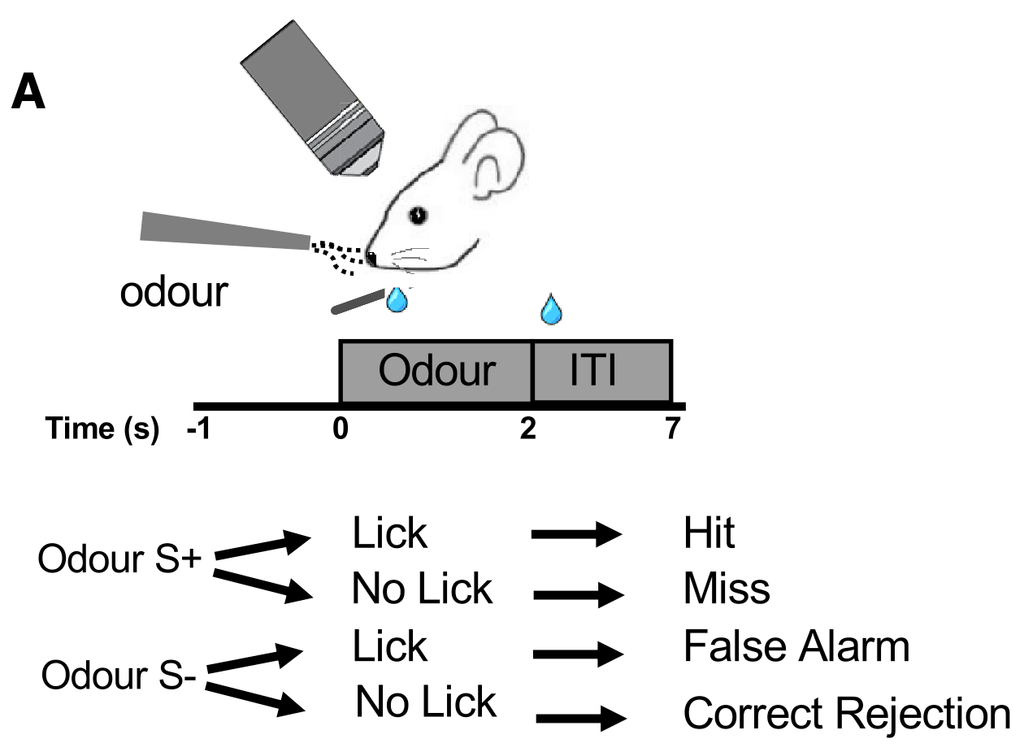
- Mouse licks water spout to initiate trial.
- 1 second later odour is delivered, for two seconds.
- Mouse has to lick at least four times in the odour window to indicate an S+ decision.
- After 2 seconds, the odour is stopped and the reward, if any, is delivered.
- Analysis is done using the imaging data within the odour window, not the reward window, to avoid confounding with reward. But it doesn’t avoid confounding with licks.
- After the trial is over, at least 5 seconds must have passed befor the mouse can initiate the next trial.
- There is no punishment on incorrect trials.
What makes the experiment interesting is the two tasks:
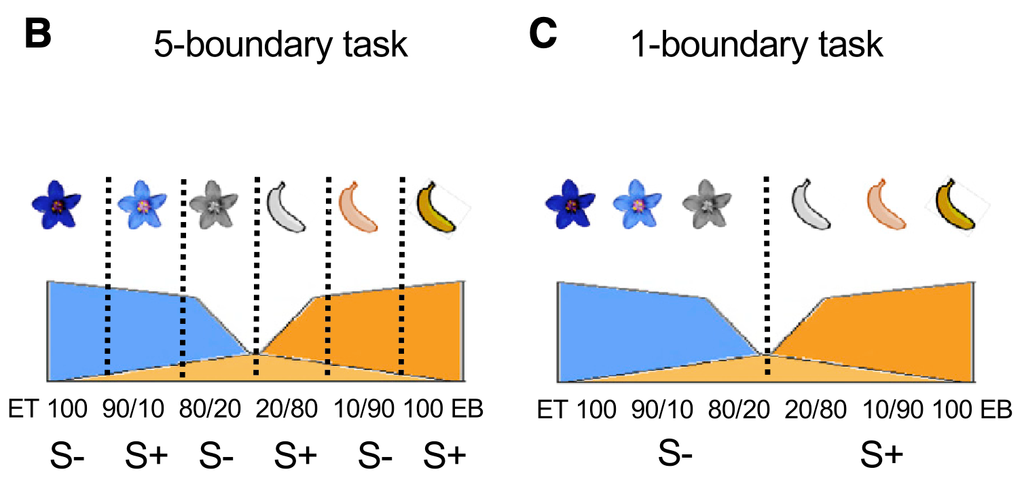
The odours are mixtures of ET and EB. In the 1b task (C), valence is determined by chemical identity alone. In the 5b task, valence is determined in a step like fashion, as if there were 5 boundaries between S+ and S-.
Importantly, notice that the inner-most and outer-most odours have the same contingency in both tasks.
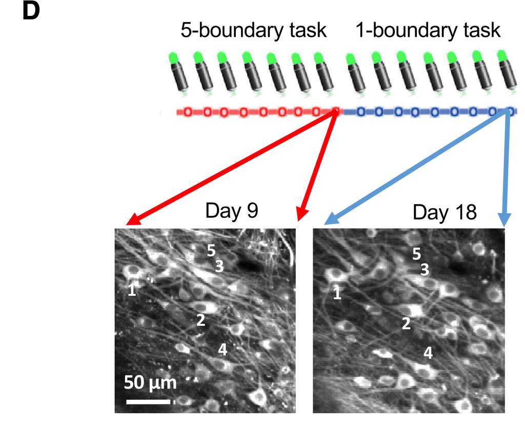
They image for 18 days: 9 days on the 5b task, then 9 days on the 1b task. Most of their results compare responses on day 9 to day 18.
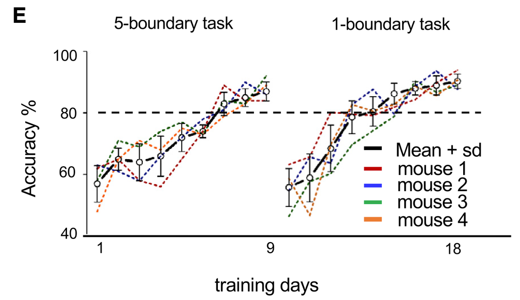
Animals seem to acquire both tasks within a few days, and to similar accuracy:
Their distribution of correct and incorrect licks is similarly distributed in both tasks:
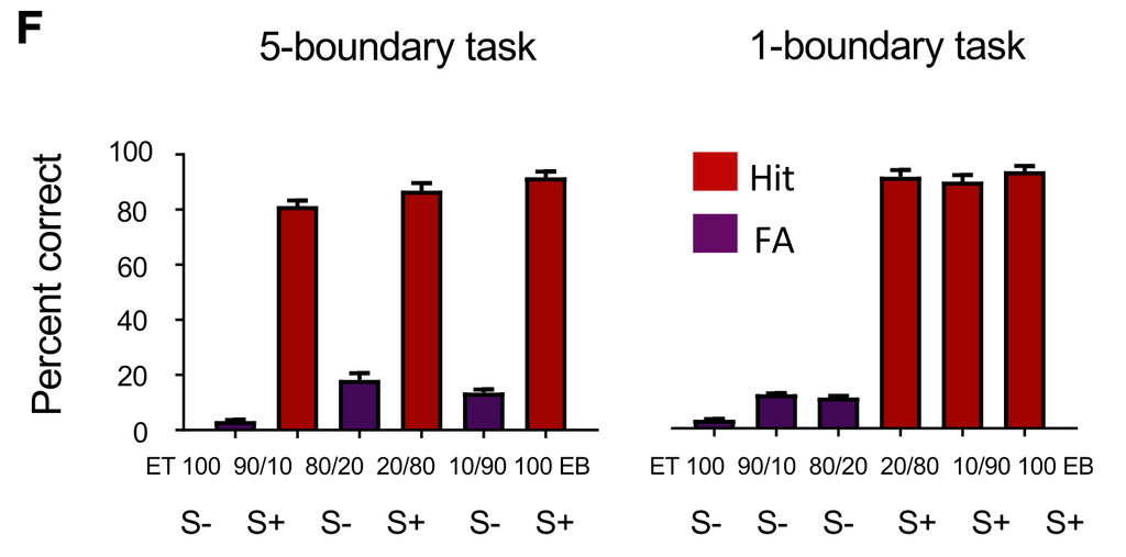
Figure 3: Task-dependent Representations
Perhaps the most striking finding of the paper are task-dependent representations: the population responses to the same odours, receiving the same reward, are different depending on the task.
The heatmaps below show the responses on the last day of the 5b task (day 9) and the 1b task (day 18). In panel A, they show the responses of cells, ordered by their correlation with the 5b template. Panel B shows the same data, but ordered by the correlation with the 1b template. The outer-most and inner-most pair of odours receive the same reward contingency in both tasks, but responses are clearly different.
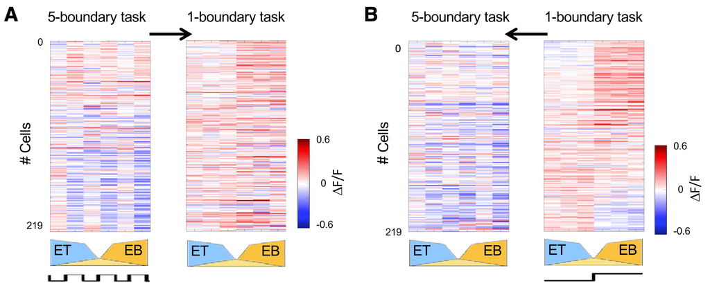
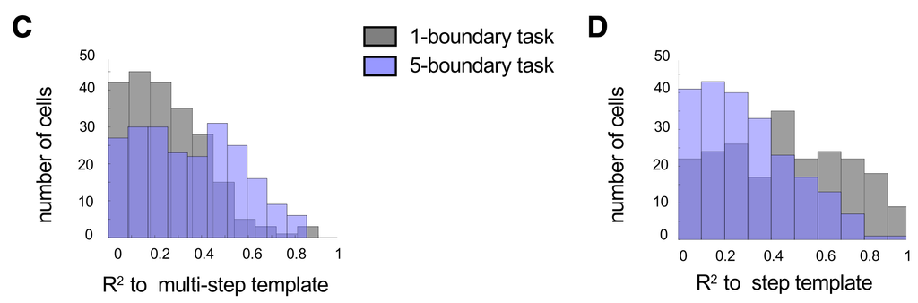
They quantify the change in representation in panels C and D, by looking at how well each template explains the response patterns in the two cases. In the 5b tasks, the multi-step template explains many of the responses well. But the same template no longer works as well in the 1b task. The reverse occurs for the step template, which doesn’t explain the 5b responses well, but explains the responses in the 1b task much better. These data indicate that the pattern of responses changes between the tasks, to reflect the task reward contingencies.
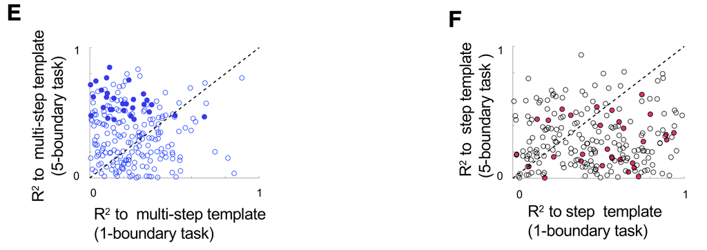
In E and F they plot the same data but for the individual MCs. Panel E measures how well the multi-step template explains the responses in the 1b (x) vs 5b (y) tasks. Most of the points lie above the diagonal, indicating the multi-step template explains the 5b task responses better. The gray and purple distributions of C are the x and y marginals of this panel. Similarly, panel F measures how well the step-template applies in the two tasks. Most of the points are below the diagonal, indicating that it explains the 1b data better. The x and y marginals here are the gray and purple distributions of panel D.
To further demonstrate how valences modulate representations, they plot the response time courses of the top 30 cells that were most step-like in the 5b task. These show that the responses to the exact same odour are modulated by its valence:
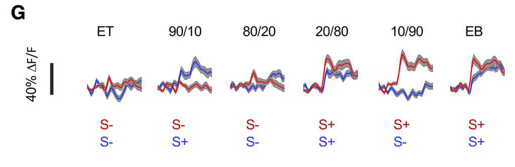
Figure 4: Population Representations
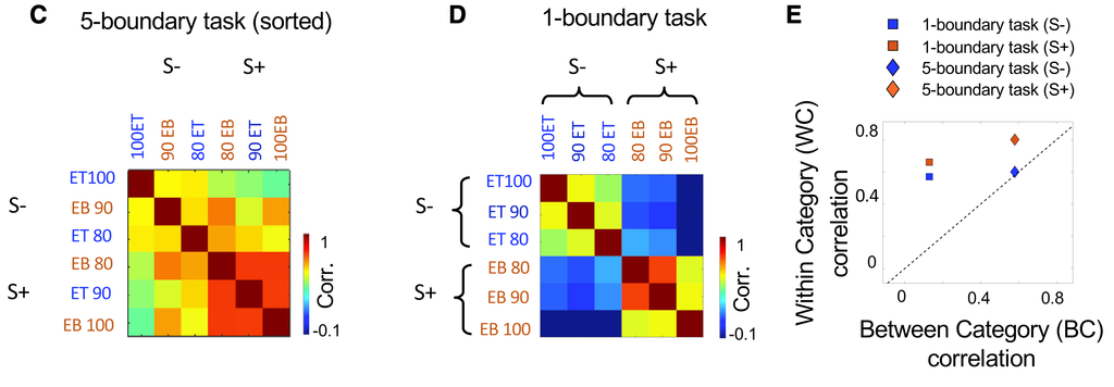
In Figure 4 they look at how odours are represented on a population level, in particular the similarity of odour responses. They find that there’s a clear grouping by valence in the 1b case, but in the 5b case, this is only for the S+ odours, the S- odours remain at the between category level of correlation.
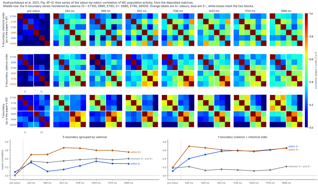
They also track how this structure develops in time. The S+ cluster establishes within ~300 ms in both tasks. The S- cluster needs till ~900 ms to establish in the 1b task. In the 5b task, it never establishes.
The animal’s performance reflected the establishment of these correlations (H, below). On low performance trials of the 5b task, the population correlations reflected chemical similarity, not valence (panel I). They quantified this using a categorization index contrasting within and between category correlations. High-performance trials had high categorization index, and conversely (J).
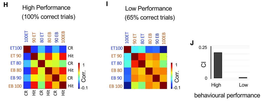
Figure 5: Decoding MC Populations
In this figure they ask what information is available in MC representations in each setting. In particular, they use linear discriminant analysis (LDA) to decode either valence (5A-F) or identity (remaining panels).
Q: Where the responses measured on the last day of each sessions?
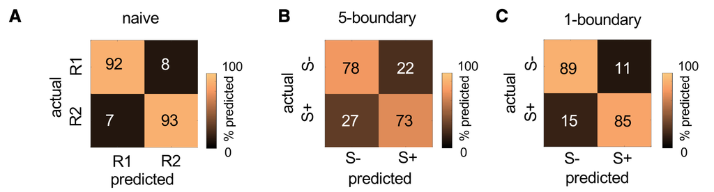
Figures 5A-C shows the confusion matrices for decoding valence (B-C) or primary odour (A?), showing good decoding accuracy in all cases, a little better in 1b than 5b:
In 5D-F they label the odours by either the 1b or 5b logic, and compare decoding accuracy using their specified logic to a shuffled control. They find in each case that labelling “correctly” (1b-logic in the 1b case, etc.) produces higher accuracy vs shuffles, while the “incorrect” labelling is indistinguishable from the shuffles.
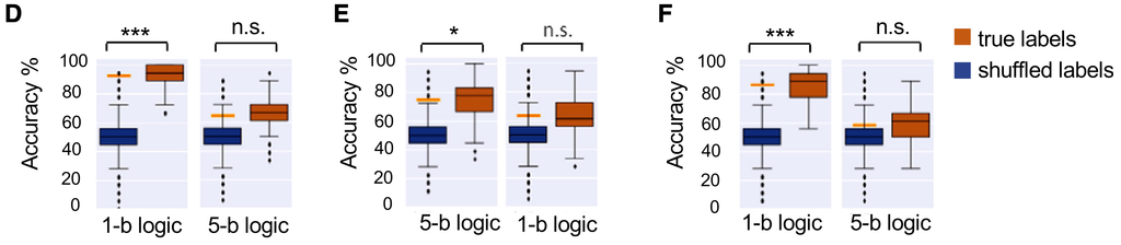
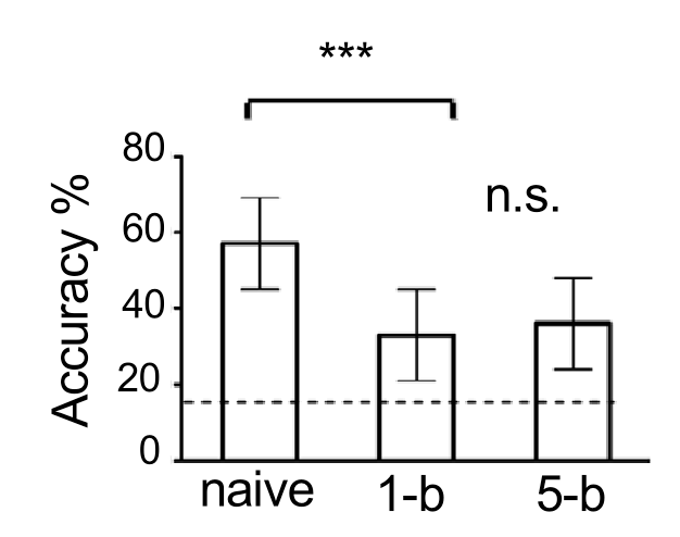
Figure 5G shows that identity decoding is diminished in both 1b and 5b cases relative to the naive condition:
The next few panels look at decoding identity.
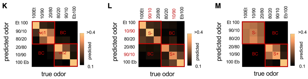
In the naive case (5K), the extreme odours are easily identified, and the intermediate odours in each category are somewhat confused, which is not surprising. In the 1b task, the S- odours are merged, while the S+ odour discriminability is similar to the naive case. Interestingly, in the 5b task (5L), the individual odours seem better discriminated than in either of the other two conditions, but 5G indicates that this is not the case, and the problem is due to the clipping by the colorbars. Claude remade the figure with an extended scale:
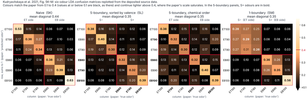
They next look specifically at the pattern of errors in each case. The results reflect the picture above – within category errors are higher than between category errors, and that the within category odours are merged more and better separted from the other category in the 1b case than in the 5b case:
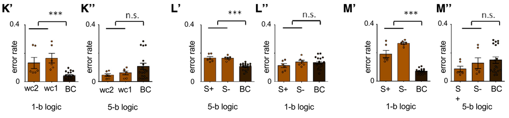
The main message of this figure is that odour representations become organized by task category rather than chemical identity.
Figure 6: Decoding Behaviour from MCs
In the next figure they see how much behavioural output can be decoded from MCs.
What’s great about their experimental design is that the innermost and outermost pair of odours have the same reward contingency in both the 1b and the 5b task. They can then compare responses to these pairs in the two tasks.
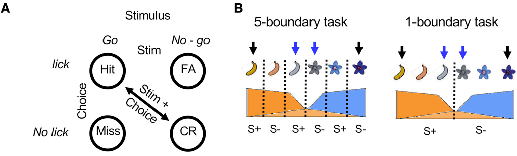
They compute discriminability on a single neuron level, by computing the AUC for the neuron as a discriminator, converting this to a discriminability score, then showing the distribution across the population.
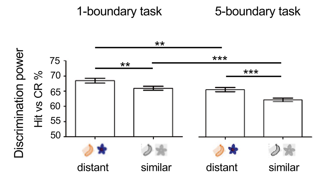
The results on correct trials (Hits vs. CR) are shown below. Distant odours are easier to discriminate than similar ones, and that discriminability gets worse in the 5b task, presumably because it’s harder. So MC responses track chemical identity and task difficulty.
Next they compared stimuli with different task outcomes in the 5b task (the 1b task didn’t have enogh error trials). Note that y-labels on E-G are incorrect.
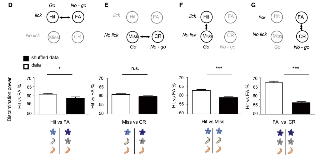
Panels D and E differ only by stimulus, and the effect is small. What makes the most difference is whether the animal licked or not (F and G).
In 6H they look at what the activity of the 30 cells most aligned to the 5b task template looks like in correct vs incorrect trials. Hit trials produce strong inhibition. And the in the S- trials which were responded to (the false alarms), the activity was also a strong inhibition, reflecting the action actually taken.
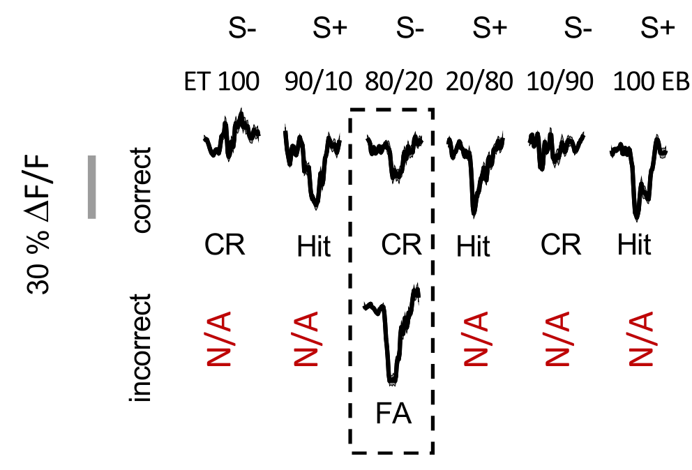
These 30 most active cells are also good discriminators for whether the animal licked or not (FA/CR, Hit/CR), and not stimulus (Hit/FA). They use these combinations because they can keep the chemistry mostly constant (CR to ET100, Hit to 90/10, FA to 80/20). The ROC curves below appear to be from the pooled responses of the 30 cells, while the histograms seem to be the distribution of AUC curves across the 30 cells.
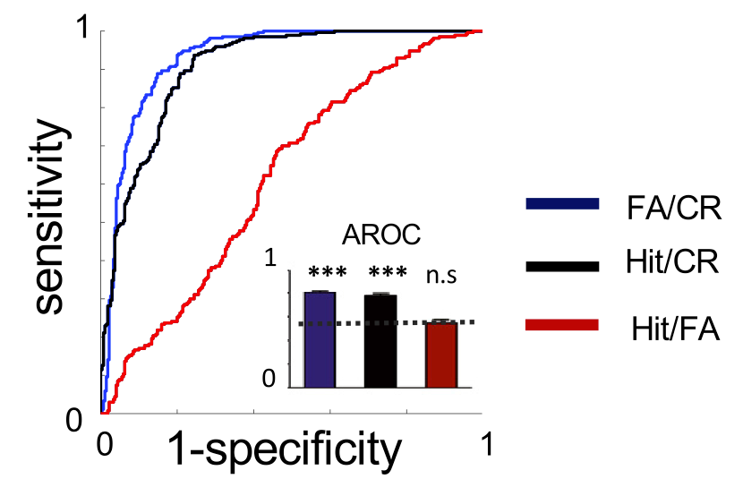
Figure 7: Reorganization of Inhibition Across Tasks
In Figure 6 we say that, at least in the 5b task, individual MCs seem particularly selective for whether the animal licked or not. In the most task-selective neurons, this inhibition seemed to manifest as additional inhibition on the S+ trials.
This could be due to a licking artifact, since the animal had to lick at least 4 times during the odour window to indicate their classification as S+, though imaging ended before water delivery.
If their MC signal is indeed a licking artifact, and nothing changes about licking between the two tasks, then we would expect a similar inhibitory response to S+ odours in the two tasks. And a different response, but again similar across the two tasks, to the S- odours.
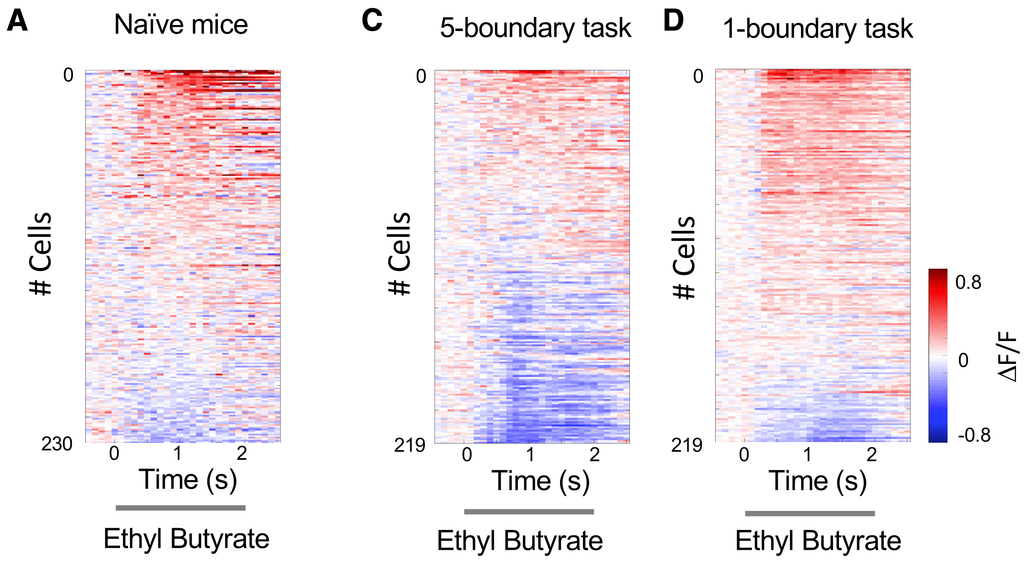
This question is what they examine in Figure 7. In particular, they examine the nature of inhibitory and excitatory responses to the S+ and S- odours in the two tasks. They find (a) that there’s more inhibition overall in the 5b task, and (b) that the S+ responses become more excitatory in the 1b task.
In 7A-C they plot the responses of 230 MCs in naive mice (A) or the same 219 MCs on day 9 (end of 5b) and day 18 (end of 1b) training, to Ethyl Butyrate, an S+ odour in both tasks. It’s clear that there’s more inhibition in both cases.
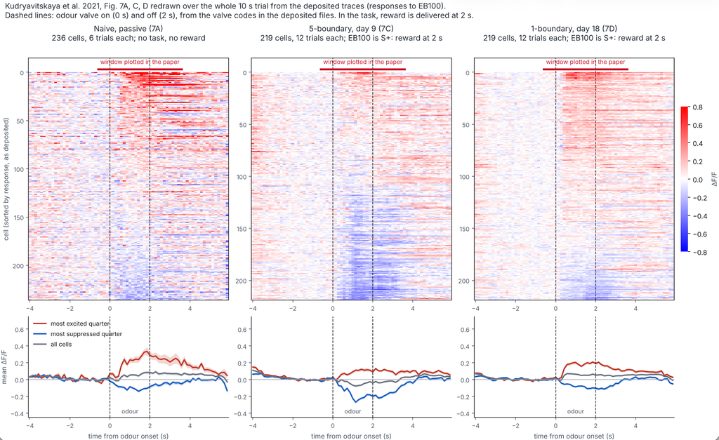
The data they provide allows us to extend these plots further into the reward period, where there might be more activity due to licking, but there isn’t an obvious change:
In 5B and E they quantified the fraction of cell-odour pairs resulting in excitatory vs. inhibitory responses. The fraction of inhibitory responses is similary between the Naive and 1-boundary case, and higher in the 5b case:
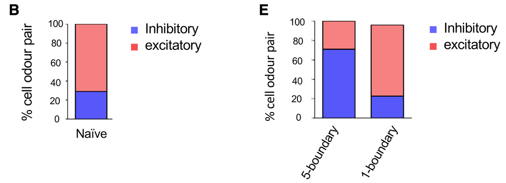
If inhibition was a licking artifact, we would expect that the 5b and 1b results to be similar. Instead, the 1b results are similar to the Naive case, which was passive exposure and did not require licking.
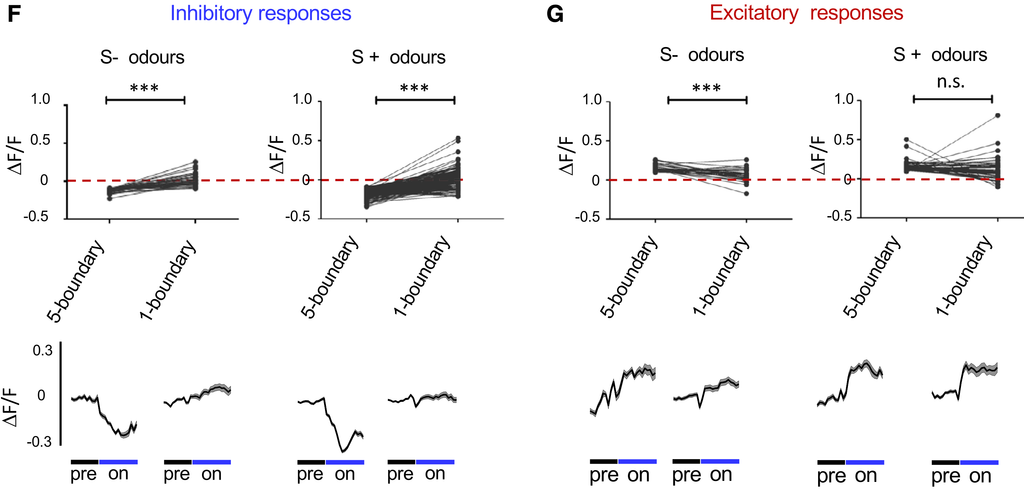
Next they grouped odour responses as excitatory or inhibitory based on their peak amplitudes relative to baseline at day 9, at the end of the 5b task. As S- odours they took the two odours that were S- in both tasks, and similarly for S+ odours. For each type of cell-odour response, they measured the change on day 18, after the 1b task. They find that both inhibitory and excitatory responses mellow, though part of this could be regression to the mean:
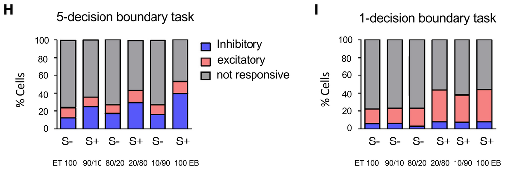
In H and I, they look at their full task-involved population of 219 MCs, and classify their responses to each odour on each task. They find again that (a) there’s more inhibition for 5b than 1b, and (b) this inhibition is focused on the S+ odours. In the 1b case there’s more excitation, especially on the S+ odours. If we focus on just the S+ odours, we see that on a population level, the response changes from inhibitory to excitatory. This is not what we would expect if responses were inhibitory licking artifacts.
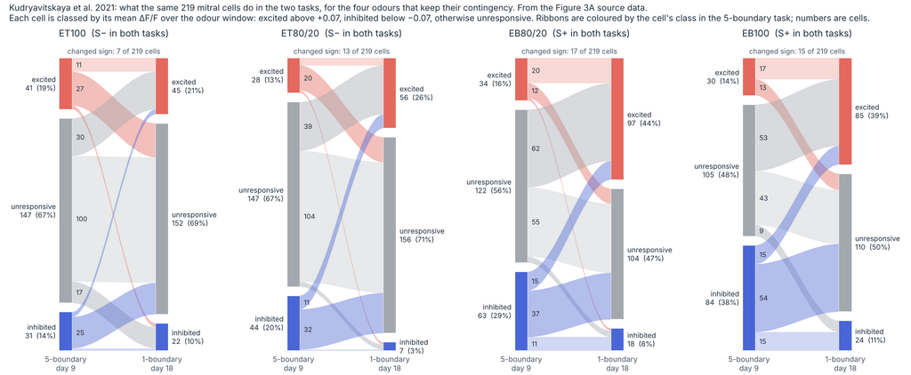
Are the same neurons involved in both types of responses when we go from the 5b to the 1b task? Below we look a this for the odours that had the same contingency in both tasks. Excitatory 1b responses seem to be recruited mainly from the silent 5b cohort. Inhibitory responses are a bit more mixed:
Leave a Reply