These are my notes fleshing out Section 5.3.3 of Bishop’s PRML, on the Efficiency of Backpropagation.
I wanted to see what makes Backpropagation so efficient. So I examined the expression in Bishop, and realized it didn’t make sense:
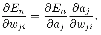
Here $E_n$, the error for one sample (I will just call it $E$ henceforth), seems to be a function of both the weights and the activations. What’s actually going on?
We can take two views of the error generated by a neural network.
The first is that it’s a function of the weights: $E(\ww)$. This is ultimately what we care about, since it’s the weights that we’ll be adjusting to reduce the error.
If we know nothing else about the structure of the network, then estimating the gradients will be expensive.
To do so, we’d need to estimate the gradient of $E$ with respect to each weight. Knowing nothing else, the way to do this is by computing finite differences. That is, computing value of the error $E(\ww + \Delta w_{ij})$ after perturbing each weight $w_{ij}$, and comparing to $E(\ww)$ to estimate the gradient. If we assume evaluating $E$ will cost on the order of the number of weights, $N^2$, then evaluating these perturbations will incur that cost once for each weight, giving an $O(N^4)$ cost.
This procedure is general, assuming only differentiability of the error function. In fact, we haven’t used any notion of neurons, networks, or activations. But the price we pay for the generality is the high cost of evaluating the gradient, which we’d have to pay at each step.
To reduce this cost, we have to introduce some structure into how the weights determine the error. So at this point we bring in neurons. Specifically, we say that the error of the network is ultimately determined by the activations of the neurons it contains. We will call this error function, which is a function of the activations $\aa$, $F$. The activations are a function of the weights, so we can say $$ E(\ww) = F(\aa(\ww)).$$
The function $\aa(\ww)$ implements the activations of the units in the network. It is defined implicitly as the solution of the activation equations. For example, we might have $$ \aa = \WW h(\aa) + \xx,$$ indicating that the activations of each unit are the sum of the inputs it receives, $\xx$, and the inputs from all the other units.
We can define the network function $$ G(\aa, \ww) = \aa – \WW h(\aa) – \xx.$$ Then $\aa(\ww)$ is defined as the (hopefully unique) value which sets this to zero: $$ G(\aa(\ww), \ww) = \bzero.$$
We can now relate the gradient of the error function with respect to the weights with that with respect to the activations, $$ {\partial E \over \partial w_{ij}} = \sum_k {\partial F \over \partial a_k} {\partial a_k \over \partial w_{ij}}.$$
The first partial derivative is straightforward. Note that it’s 0 for the hidden units, since the error only depends on whatever units we decide are output units.
To compute the partial derivatives of the activations with respect to a given weight, we perturb the weights to the network function and look for activations that keep it at zero:
$$ G(\aa + \Delta \aa, \ww + \Delta w_{ij}) \approx G(\aa, \ww) + G_a \Delta \aa + G_{w_{ij}} \Delta w_{ij}.$$
Since both network functions are 0, we get $$ G_a \Delta \aa + G_{w_{ij}} \Delta w_{ij} = 0 \implies \lim_{\Delta w_{ij} \to 0} {\Delta \aa \over \Delta w_{ij}} = {\partial \aa \over \partial w_{ij}} = -G_a^{-1} G_{w_{ij}}.$$
We then arrive at $$ {\partial E \over \partial w_{ij}} = – \nabla_\aa F^T G_a^{-1} G_{w_{ij}}.$$
What does this look like for our network function above?
\begin{align*} G_a &= \II – \WW \DD, &\quad& \DD = \diag(h'(\aa)) \\ G_{w_{ij}} &= -e_i z_j, &\quad& z_j = h(a_j). \end{align*}
What is the cost of this computation?
First, we need to determine the activations. That involves finding an $\aa$ that satisfies the network equation. In the simplest case of linear activations, we still need to solve $$ (\II – \WW)\aa = \xx.$$ This requires inverting the matrix on the left-hand-side, an $O(N^3)$ computation.
Let’s assume that with the activations in hand, $F(\aa)$ is a simple function with an easy gradient. E.g. if we’re using squared-error loss, we have something like $F(\aa) = \sum_{i \in \text{output}} (a_i – y_i)^2,$ then the gradient is simply proportional to $(\aa – \yy)$, linear in the number of units. So let’s assume that, given the activations, $\nabla_\aa F$ has $O(N)$ cost.
The $G_a^{-1}$ term also requires inverting an $N \times N$ matrix, an $O(N^3)$ computation.
Multiplying the gradient with this inverse involves $N$ multiplications plus a sum of $N$ terms per column of $G_a^{-1}$, so an $O(N)$ computation, $N$ times, for a total of $O(N^2)$.
Thus, determining $\nabla_a F^T G_a^{-1}$ is an $O(N^3)$ computation, that only has to be done once per round of weight updates. The individual weight updates are found by multiplication of this vector with $e_i z_j$, which amounts to multiplying its $i$’th element by the output of the $j$’th unit, i.e. an $O(1)$ computation given what’s already been computed.
Therefore, even in the case of linear activation functions, the weight updates incur an $O(N^3)$ cost because of the matrix inversions required.
The cubic cost of the updates reflects the possibility of feedback connections in the network. Determining the activations or their gradients requires matrix inversions that account for these feedback connections, and because we’ve allowed our weight matrix to be fully general, there is no shortcut to performing the inversion.
However, if we limit our weight matrices to be feedforward, then an efficient solution exists: forward substitution.
Feedforward connectivity means there’s an ordering of the units where units only connect to other units that have a higher ordering. The corresponding connectivity matrix, where rows are targets and columns are sources, would be strictly lower triangular.
To see how this would work, recall the network equation that we have to satisfy $$ \aa = \WW h(\aa) + \xx.$$ Now start at the first unit. Because it’s the first unit, it only receives external input, so $$a_1 = x_1,$$ and its activation is determined.
The second unit receives external input, but also input from the first unit, $$a_2 = x_2 + w_{21} h(a_1),$$ where $h$ is the activation function. Since we already have $a_1$ above, we can substitute that in, and thereby determine $a_2$. Continuing in this way, we get $$a_n = x_n + \sum_{i<n} w_{ni} h(a_i).$$
Computing the first activation requires one operation, the second, two operations, the third, three operations and so on. Therefore, by allowing activations to percolate from the earliest units forward, we only need $O(N^2)$ operations, instead of $O(N^3)$ to compute the forward pass and arrive at the activations. We’ll assume that the gradient of $F$ with respect to the activations will incur the same $O(N)$ cost as before.
Next we come to $G_a^{-1}$. Notice that we don’t need the inverse, just a particular application of it, since $$ \nabla_a F^T G_a^{-1} = \delta^T \implies G_a^T \delta = \nabla_a F.$$
Now $G_a = \II – \WW \DD$ is lower triangular, so $G_a^T$ will be upper triangular. We can therefore start at the `bottom’, i.e. the output-most unit, and apply backward substitution, i.e. backpropagation, to determine the elements of $\delta$ from the outside in, incurring an $O(N^2)$ cost.
Then, returning to our expression for the gradient of the error with respect to the weights, we have $$ {\partial E \over \partial w_{ij}} = -\nabla_a F ^T G_a^{-1} G_{w_{ij}} = \delta^T e_i z_j = \delta_i z_j.$$
We’ve seen above that the computation of $\delta$ has $O(N^2)$ complexity, and that of the activations and outputs also has $O(N^2)$ complexity. The individual updates then only involve an $O(1)$ product of pairs of terms, one from each. Therefore, the overall cost of the gradient updates is $O(N^2)$.
Summary
In summary we can trace the efficiency of backpropagation to two items:
- Expression of the error as a function of the output units of a network. This reduced the cost in our example from $O(N^4)$ to $O(N^3)$, for a linear network.
- Restricting the connectivity to be strictly feedforward. This allowed us to compute forward and backward passes in $O(N^2)$ time.
The derivation also reveals that these results generalize beyond the standard feedforward networks in which units in one layer connect only to units in the next layer. We’ve seen above that all we need is lower triangular structure in the weight matrix, which means an ordering of the units in which earlier units only project to later ones. This allows elaborations of standard feedforward networks – for example, within-layer connections (as long they’re acyclic), or skip connections from one layer to units more than one layer ahead.
Postscript: Returning to Bishop
So hopefully we now have a mathematically coherent understanding of how backpropagation works and why it’s efficient.
But we had to do a bit more work than Bishop does to arrive at the same point, and his expression makes sense on its own terms. How do we reconcile our approach with his?
Let’s recall his expression: $$ {\partial E \over \partial w_{ij}} = {\partial E \over \partial a_i} {\partial a_i \over \partial w_{ij}}.$$
The expression makes intuitive sense: $w_{ij}$ only affects $a_i$, so the effect of $w_{ij}$ on the error can only go through $a_i$.
And the partial derivative of $a_i$ with respect to $w_{ij}$ is easy to justify as a real partial derivative of the function $$a_i(w_{i1}, \dots, w_{i,i-1}, a_1, \dots a_{i-1}) = \sum_{j=1}^{i-1} w_{ij} h(a_j).$$
This just expresses the feedforward structure of the network. The partial derivative is easy to read off as $h(a_j) = z_j$.
But what is ${\partial E \over \partial a_i}$? It seems to be the entire downstream effect of perturbing $a_i$ on the error. And it makes sense to decompose it as $$ {\partial E \over \partial a_i} = \sum_{k > i} {\partial E \over \partial a_k} {\partial a_k \over \partial a_i}.$$
This says the downstream effects can be defined recursively in terms of the units that $a_i$ drives.
$$\blacksquare$$
Leave a Reply