Grokking as Lazy-to-Rich Learning

These are my notes on some of the key results in Kumar et al.’s “Grokking as the Transition from Lazy to Rich Dynamics.”

What is Grokking

Grokking was the observation made by Power et al. who trained small transformers on modular arithmetic and related tasks, of a large gap between training accuracy and test accuracy reaching 100%:

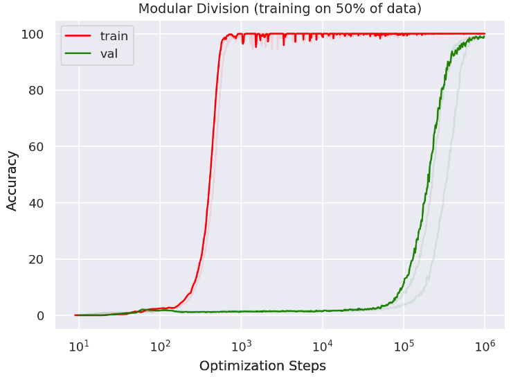
Although training accuracy reaches 100% early, it takes 3 orders of magnitude more iterations before the network “grok”s the problem, and test accuracy starts to rise. Why does this occur?

Lazy Learning

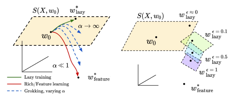
The solutions suggested by Kumar and colleagues is that grokking reflects the transition from a “lazy” learning regime, in which the network tries to fit the training data without moving too far from its initialization, to a “rich” regime, in which the network finally moves outs of the neighbourhood of its initialization, and learns task-relevant features, which generalize to the test set.

The basic idea is that we can always view learning by gradient descent locally as a regression problem, whose kernel determines directions that are easy (large eigenvalue) and hard (small eigenvalue) to learn. The lazy regime corresponds to learning along the easy directions around the initial point.

Let’s get concrete. We’re studying a regression problem, where we’re minimizing $$ L(\ww) = {1\over 2N} \sum_i (y(\xx_i) – f(\ww, \xx_i))^2.$$ We do this using gradient descent, so $$ \dot \ww \propto -\nabla_\ww L = {1 \over N} \sum_i (y(\xx_i) – f(\ww, \xx_i)) \nabla_\ww f(\ww, \xx_i).$$

The weights start at $\ww_0$, and we can consider the infinitesimal motion around initialization. Since the weight updates will be infinitesimal, we can write \begin{align*} f(\xx, \ww) &= f(\xx, \ww_0) + \nabla_\ww f(\xx,\ww_0) (\ww – \ww_0)\\ &= f(\xx, \ww_0) – \nabla_\ww f(\xx, \ww_0) \ww_0 + \nabla_\ww f(\xx,\ww_0) \ww . \end{align*} So infinitesimal changes around an initial value are affine in $\ww$: $$ f(\xx, \ww) = b(\xx, \ww_0) + \phi(\xx)^T \ww,$$ where we’ve defined the feature map $$ \phi(\xx) \triangleq \nabla_\ww f(\xx, \ww_0).$$

In these terms, the weight dynamics are $$ \dot \ww = {1 \over N} \sum_i (y(\xx_i) – \phi(\xx_i)^T \ww) \phi(\xx_i),$$ where we’ve absorbed $b(\xx_i,\ww_0)$ into $y(\xx_i)$ since it doesn’t depend on $\ww$. So, weight dynamics around initialization are linear regression.

If we stack the features into a matrix as $$ \bPhi \triangleq [\phi(\xx_1), \phi(\xx_2),\dots,\phi(\xx_N)],$$ then we can write the weight update as $$ \dot \ww = \bPhi (\yy – \bPhi^T \ww).$$

We’re studying large networks, so $\ww$ can have very high dimensionality. We can instead study the much more tractable object, the predictions, $\aa = \bPhi^T \ww$. These change as $$ \dot \aa = \bPhi^T \bPhi \yy – \bPhi^T \bPhi \aa = \KK \yy – \KK \aa,$$ where $$ \KK \triangleq \bPhi^T \bPhi, \quad K(\xx, \xx’) = \phi(\xx)^T \phi(\xx),$$ is the kernel of the regression, the neural tangent kernel in our case.

We can eigendecompose the kernel as $$ \KK = \UU \SS^2 \UU^T.$$ If we switch coordinates to these eigenvectors, so $\tilde{\aa} = \UU^T \aa,$ then $$ \dot{\tilde{a_i}} = S_i^2 \tilde{y_i} – S_i^2 \tilde{a}_i.$$

This equation says two things:

1. The predictions along the principal eigenvectors of the kernel, those for which $S_i$ is large, are learned faster than those along other directions. Lazy learning cooresponds to learning along these directions, as defined around the initial conditions.
2. We want those directions to lineup with $y$. It doesn’t matter if we have fast decay along some directions, if our targets don’t lie along those directions.

The second point motivates using centered kernel alignment, CKA, as a measure of how well the kernel can capture the targets: $$\text{CKA} = { \yy^T \KK \yy \over \|\KK\| \|\yy\| } = {\sum_{i=1}^P \tilde{y}_i^2 S_i^2 \over \| \KK \| \| \yy \|}.$$ The numerator is a projection of $\yy$ along the eigenvectors of $\KK$, weighted by the eigenvalues, literally measuring alignment. The denominator normalizes the value to lie between 0 and 1.

CKA also measures how quickly the loss initially drops. Since $L = {1 \over 2 N} \| \yy – \ff(\ww, \xx)\|_F^2,$ $$ {dL \over dt} = -{1 \over N} (\yy – \ff)^T \dot \ff.$$ At the start of learning, we’re in the lazy regime, so $\ff(\xx, \ww) = \ff(\xx, \ww_0)$, so $\yy – \ff = \yy – \ff(\xx, \ww_0)$, which we abused notation and also called $\yy$. Also, $\dot \ff = \dot \aa$. So we get $$ {dL \over dt} = -{1\over N} \yy^T \dot \aa = -{1 \over N} \yy^T \KK \yy,$$ which is the numerator in CKA.

Polynomial Regression

To demonstrate how lazy vs rich learning explains grokking, the authors study a simple polynomial regression problem. Instead of using a transformer, they study a two layer network with fixed output weights. So their network output is $$ f(\ww, \xx) = {\alpha \over N} \sum_{i=1}^N g(\ww_i^T \xx),$$ where $\xx \in \RR^D$, and $g$ is a polynomial activation function.

Previous work by others has shown that when the activation function is an order $k$ polynomial, the functions can be learned using as many examples $P$ as the dimensionality of the input $D$. The authors’ previous work has shown that lazy learning requires $D^k$ examples, where $k$ is the oder of the nonlinearity. This gap suggested that grokking was possible.

To determine the lazy and rich directions, the authors comptued the NTK for the regression problem, using quadratic activation function $$g(h) = h + {\veps h^2 \over 2}.$$ To compute the NTK we need the partial derivatives of the output $f$ relative to the weights. These split in $N$ independent blocks, one for each hidden unit. The component from block $i$ is $$ {\partial f \over \partial \ww_i} = {\alpha \over N} g'(\ww_i^T \xx) \xx = {\alpha \over N} (1 + \veps \ww_i^T\xx) \xx.$$

The kernel measures how these features overlap for different inputs, \begin{align*} K(\xx, \xx’) &= \phi(\xx)^T \phi(\xx’)\\ &= \sum_i {\partial f (\xx, \ww_0) \over \partial \ww_i}^T {\partial f (\xx’, \ww_0) \over \partial \ww_i} \\ &= {\alpha^2 \over N^2} \sum_i (1 + \veps \ww_i^T \xx)(1 + \veps \ww_i^T \xx’) \xx^T \xx’ \\ &={\alpha^2 \over N^2} \left[ N \xx^T \xx’ + \veps \sum \ww_i^T (\xx + \xx’) \xx^T \xx’ + \veps^2 (\xx^T \xx’) \xx^T \sum_i \ww_i \ww_i^T \xx’ \right]\\ &= {\alpha^2 \over N} \left[ \xx^T \xx’ + \veps \overline \ww (\xx + \xx’) \xx^T \xx’ + \veps^2 \xx^T \MM \xx (\xx^T \xx’)\right],\end{align*} where $$ \overline \ww \triangleq {1 \over N} \sum \ww_i, \quad \MM \triangleq {1 \over N} \sum \ww_i \ww_i^T.$$

At their initialization $\overline \ww = \bzero$ and $\MM = \II$. So, ignoring the constantant of proportionality, $$K_0(\xx, \xx’) = \xx^T \xx’ + \veps^2 (\xx^T \xx’)^2.$$

Now for a given dataset, $K_0$ will have a specific value and will give us some specific eigenvectors that will be easy or hard to learn. We’ll get more insight if we consider these eigenvectors in the limit of infinite data.

To do that, let’s write the eigenvector equation in the finite data case: $$ {1 \over P} \sum_\nu K(\xx_\mu, \xx_\nu) r^{(a)}_\nu = \lambda^{(a)} r^{(a)}_\mu.$$