Notes on Toy Models of Superposition

On the Discord we’ve been discussing “Toy Models of Superposition” form Anthropic. It’s a long blog post, so these are my running notes to get people (and myself) up to speed if they’ve missed a week or two of the discussion.

Problem Setup

The authors’ basic aim is to demonstrate “superposition“: neurons representing multiple input features.

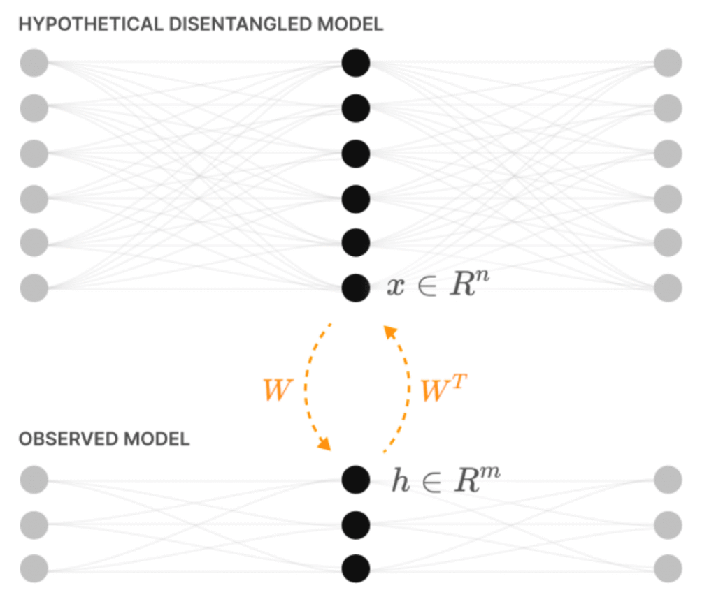
They bring this about by considering the compression of high-dimensional input features into a low dimensional hidden layer, and then back again. Because of their interest in interpretability, they imagine the high-dimensional features correspond to the disentangled representations of the environment that a hypothetical very large neural network would use. Such a network would be able to explain its sensory input as the presence of a number of features that correspond to interpretable aspects of the environment.

In this larger network, each hidden layer neuron represents one feature. In a smaller network, the hidden layer neurons have to represent multiple features, producing superposition.

They study the input features that each hidden layer neuron responds to, and how this changes as the statistics of the input are altered.

Model and Loss

For most of the paper they consider two flavours of model. One is purely linear, the other applies a ReLU at the output to clean up the responses:

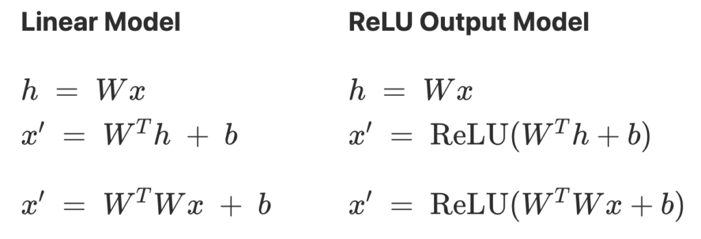
They optimize the weights $W$ to minimize the importance weighted loss,

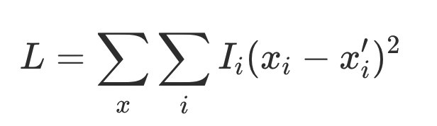
The feature importances $I_i$ are typically set to exponentially decay so as to put more importance on the first few features. For example $I_i = 0.7^i$.

Geometry of Superposition

Uniform superposition

To simplify the study they first consider uniform feature importance.
- $I_i = 1$ for each of the $n=400$ input features.
Learned features has approximately unit norm, so quantified number of learned features as $\sum_{i=1}^n \|W_i\|_2^2 = \|W\|_F^2.$
Measured superposition using Dimensions per Feature, $$ D \triangleq {m \over \|W\|_F^2}.$$
The lower this number, the more input features are being crammed into the $m$ hidden units, hence more superposition.
Found, as expected, that $D$ decreases with sparsity, implying more superposition. Interestingly, the plot also had plateaus.
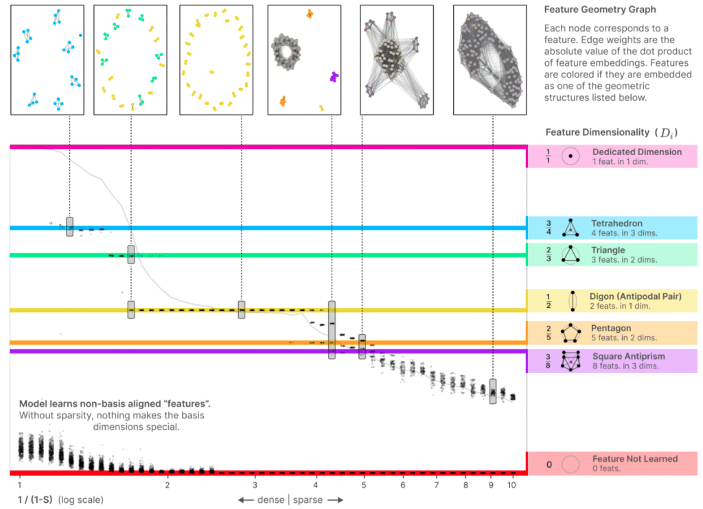
Defined the feature dimensionality to measure how much each feature overlaps with the others $$D_i \triangleq {\|W_i\|_2^2 \over \sum_j (\hat W_j \cdot W_i)^2}.$$
Feature dimensionalities indicate geometric configurations of features.
- If a feature doesn’t overlap with any others, $D_i = 1$.
- If it overlaps with an antipodal feature, $D_i = {1 \over 1 + 1} = {1 \over 2}$, etc.
Overlaid the dimensions per feature plot (trace) with the feature dimensionalities (dots), and saw that plateaus corresponding to particular geometric configurations of features:

Non-uniform Feature Importance

They considered making one of the 5 input features more or less important than the others.
As that feature decreased in importance, the lowest energy configuration transitioned from the pentagon to the diamond (digon):

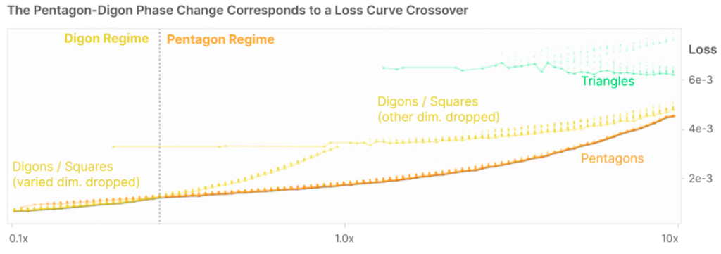
This makes sense – if an input feature is not very important to reproduce, the network will eventually drop it.

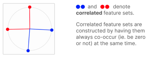
Correlated and Anti-Correlated Features

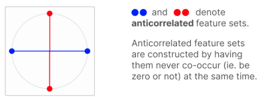
Tried situations where features were correlated (always co-occur) or anti-correalted (one is present when the other is absent).
Correlated features tend to be have orthogonal features:

Anti-correlated features tend to be anti-podal:

Correlated features form “Local orthogonal bases”:

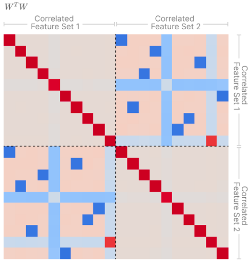
All of these effects make intuitive sense:
- if features co-occur, we want to make them orthogonal to reduce overlap, reducing superposition.
- If they’re anti-correlated we can pack them into the same directions in space, increasing superposition.

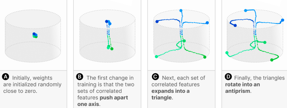
Superposition and Learning Dynamics

Looking at $n = 6$ features compressed into $m = 3$ dimensions.
Features were two groups of three correlated features.
Optimization loss has plateaus, corresponding to qualitative changes in geometry:

Superposition in a Privileged Basis

Most of the results so far have a rotational redundancy.
This is because what matters to the loss is not the weights, $W$, but their overlap $W^T W$.
Therefore, any rotation $R$ in the latent space would produce the same loss.
- Because $(R W)^T R W = W^T R^T R W = W^T W.$
This means that the weights themselves aren’t meaningful, hence why we’ve been looking at $W^T W$ throughout.
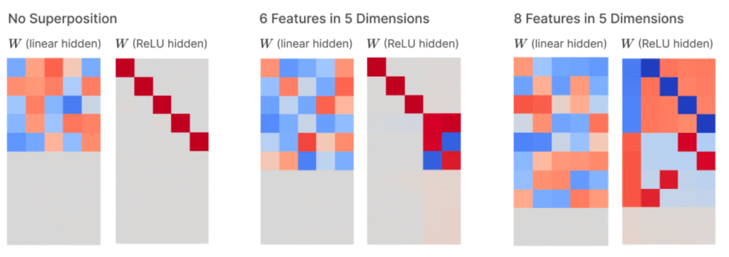
In this section the authors introduce a privileged basis by applying a ReLU at the hidden layer.
- So $h = ReLU(W x \dots).$
They find that the mapping from input features to hidden layer activations becomes interpretable.
Dense inputs produce monosemantic neurons.
Polysemanticity increases with the sparsity of the inputs.

Computation in Superposition

The aim of this section was to see whether and how useful computations can be performed in superposition.

The computation they chose was computing the absolute value of the inputs. This aligns well with the ReLU nonlinearity, since we can compute $|x|$ as $$|x| = \text{ReLU}(x) + \text{ReLU}(-x).$$

Here we can think of the two ReLUs above being computed by separate hidden units, and combined in the output. This motivated an architecture where the hidden layer activations were just like in the original setting, a linear combination of the inputs, but then with a ReLU applied. The outputs were computed from the hidden layer as before: linear combination followed by ReLU. The final difference to the original setting was that they allowed the input and output features to be learned separately. Putting it all together, the model was $$ h = \text{ReLU}(W_1 x), \quad \hat x = \text{ReLU}(W_2 x + b).$$ Inputs were as before, tested in various sparsity regimes. The only change here was that when an input was non-zero, it was sampled uniformly from $[-1, 1]$ to expose the operation to negative values.

They first tested whether their model could learn the “natural” solution we described above. So they trained a network with twice as many hidden layer units as inputs. And indeed, they found the expected solution:

Each column here represents one hidden layer neuron. The colours represent the there input features (elements of $x$). The two rows of the histogram indicate the input weights to each unit, and the output weights. So, for example, the first hidden neuron weights the first input feature at +1, and outputs +1 to the red output unit. The second hidden neuron weights the first input with -1, and outputs +1 to the red output unit. Therefore, the input the red output unit is $$ u_1 = ReLU(x_1) + ReLU(-x_1) = |x_1|,$$ and produces the correct output even without needing a further cleanup.

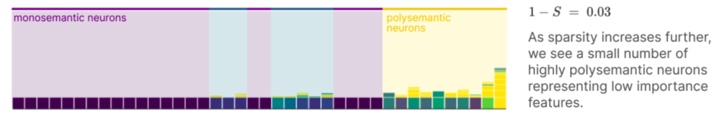
In the setting above there were two hidden units per input feature, so no superposition was required. To observe the effects of superposition, they next tried a setting with less than half as many hidden units as input features. They additionally weighted the earlier features to be more important than later ones. They found, as before, that when inputs are dense, all hidden layer neurons are monosemantic (represent one feature). When inputs are very sparse, all hidden layer neurons are polysemantic, representing multiple features. For intermediate sparsity levels, they found a mixture, with the most important features tending to be represented monosemantically:

How is absolute value computed in superposition? In addition to the “natural” solution above, they found an interesting motif they called “asymmetric superposition.”

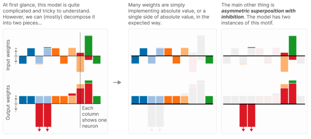
It’s a bit complicated and their explanation is not super clear so we’ll go through it step by step.

Start with the plot on the left. We have 10 hidden layer neurons (the columns), responding to 6 features (the colours).

Some of the computation is as before (middle panel). For example, consider the dark blue feature. It has two hidden layer neurons encoding it, one with positive weight and one with negative weight. These combine with equal positive weight to the darkblue output features, giving us the natural solution for that input feature. A similar thing is done for the light blue and dark orange feature.

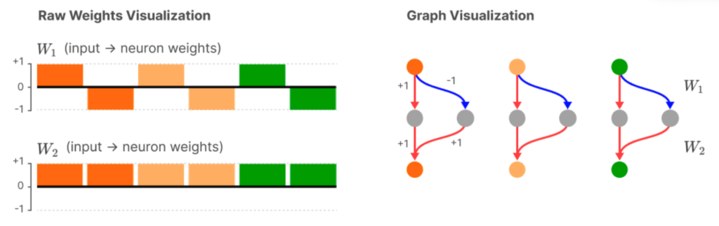
The interesting bit is how the light orange and red features are computed. The asymmetric inhibition motif they identify looks like this:

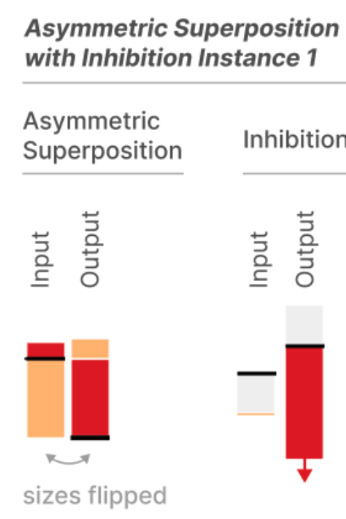
The first hidden unit, on the left, receives light positive input from the red feature, and drives the red output feature strongly. However, it receives very large negative weight from the light orange feature, which means the hidden unit will also be strongly driven when the pale orange feature has a negative value. So, the red output unit will not only be driven when the red feature is present, but also when the pale orange feature is present with a negative value.

To counteract this interference, there’s a second hidden unit, which receives a slight amount of negative input from the pale orange feature. But this hidden unit strongly inhibits the red output unit.

The net effect is that when the pale orange input is present (with a negative value), the erroneous excitation the red output unit receives from the first hidden unit is cancelled by the inhibition it receives from the second hidden unit.