These notes closely follow section 3.5 of Bishop on the Evidence Approximation, much of which is based on this paper on Bayesian interpolation by David MacKay, and to which I refer to below.
Motivation
We have some dataset of inputs $\XX = \{\xx_1, \dots, \xx_N\}$ and corresponding outputs $\tt = \{t_1, \dots, t_N\}$, and we’re interested in predicting the value $t$ of the output given a new input $\xx$. Our uncertainty in the output is determined by marginalizing over the parameters $\ww$ and hyperparameters $\alpha$ and $\beta$ of our model,
$$ p(t|\xx, \XX, \tt) = \int\int \int p(t|\xx,\ww, \beta) p(\ww|\XX, \tt, \alpha, \beta) p(\alpha, \beta|\XX, \tt) d\ww\,d\alpha\,d\beta.$$
The difficulty is that even for a simple Gaussian model mapping inputs to outputs, this full integral is not analytically tractable. Many of the references developing the evidence approximation are from the early 90s or earlier when numerical evaluation was perhaps also difficult. We are therefore looking for an approximation to this integral.
The idea of the evidence approximation is to assume that the posterior distribution of the hyperparameters $\alpha$ and $\beta$ is sharply peaked around its maximum value. If we can approximate $$ p(\alpha, \beta | \XX, \tt) \approx \delta(\alpha – \hat \alpha) \delta (\beta – \hat \beta),$$ then our triple integral simplifies to one just over the parameters $\ww$,\begin{align} p(t|\xx, \XX, \tt) &\approx \int\int \int p(t|\xx,\ww, \beta) p(\ww|\XX, \tt, \alpha, \beta) \delta(\alpha – \hat \alpha) \delta(\beta – \hat \beta) d\ww\,d\alpha\,d\beta\\ &= \int p(t|\xx,\ww, \hat \beta) p(\ww|\XX, \tt, \hat \alpha, \hat \beta)d\ww,\end{align} which, at least in a simple Gaussian model, we can analytically evaluate.
Evaluating the Model Evidence
To maximize the posterior on hyperparameters, we first assume that the prior on the hyperparameters is approximately flat, so $$ p(\alpha, \beta | \XX, \tt) \propto p(\alpha, \beta) p(\tt,\XX| \alpha, \beta) \propto p(\tt, \XX|\alpha, \beta).$$
The last term is the model evidence or the marginal likelihood. It’s called the marginal likelihood because it expresses the likelihood that the hyperparameters $\alpha$ and $\beta$ produced the data, after marginalizing out the the model parameters,
$$ p(\tt, \XX | \alpha, \beta) = \int p(\tt , \XX| \ww, \alpha, \beta) p(\ww| \alpha, \beta)\, d\ww.$$
To compute this, we need to specify our model of how inputs generate outputs.
We assume that input-output pairs are generated independently, and that outputs are a linear combination of input features, corrupted by additive Gaussian noise of precision $\beta$, so
\begin{align}
p(\tt, \XX | \ww, \alpha, \beta) &= \prod_{i=1}^N p(t_i | \xx_i, \ww, \beta) p(\xx_i) \propto \prod_{i=1}^N \mathcal{N}(t_i| \ww^T \phi(\xx_i), \beta^{-1}),\end{align} where the proportionality is through the probability of the inputs $p(\xx_i)$, which we assume are independent of the parameters and hyperparameters.
We assume a simple isotropic Gaussian prior on the weights with precision $\alpha$,
$$ p(\ww|\alpha) = \mathcal{N}(\ww|0, \II \alpha^{-1}).$$
Combining these pieces we get
$$ p(\tt | \XX, \alpha, \beta) = \sqrt{\beta \over 2 \pi}^N \sqrt{\alpha \over 2\pi}^M \int e^{-E(\ww)} \, d\ww,$$ where we’ve divided both sides by $p(\XX)$, yielding the conditional distribution on the left-hand-side. We’ve also defined
$$ E(\ww)= {\beta \over 2} \|\tt – \bPhi \ww\|_2^2 + {\alpha \over 2} \ww^T \ww = \beta E_D(\ww) + \alpha E_W(\ww).$$
To compute the integral we complete the square and express $$ E(\ww) = E(\mm_N) + {1 \over 2}(\ww – \mm_N)^T \SS_N^{-1}(\ww – \mm_N),$$ where $$\mm_N = \beta \SS_N \Phi^T \tt, \quad \SS_N^{-1} = \alpha \II + \beta \Phi^T \Phi,$$ are the posterior mean and precision on the weights given the data and the hyperparameters. This has the pleasing interpretation that the change in energy relative to the minimum at the posterior mean, is proportional to the distance from the mean, measured in coordinates given by the posterior covariance.
The integral then evaluates to $$ \int e^{-E(\ww)} \, d\ww = e^{-E(\mm_N)} \sqrt{2\pi}^M \sqrt{|\SS_N|}.$$
Putting the pieces together, we get
$$ \log p(\tt | \XX, \alpha, \beta) = {M \over 2} \log \alpha + {N \over 2} \log \beta – E(\mm_N) – {1 \over 2} \log |\SS_N^{-1}| – {N \over 2} \log (2 \pi).$$
MacKay provides an interesting interpretation of this equation in Section 4 of his paper. If we expand $E(\mm_N)$ we can write the log evidence as $$ \log p(\tt |\XX,\alpha, \beta) ={N \over 2} \log {\beta \over 2\pi} – \beta E_D(\mm_N) – \alpha E_W(\mm_N) – {1 \over 2} \log {|\SS_N^{-1}| \over \alpha^M}.$$
The $-\beta E_D$ term is the negative of the sum of squares of the residuals of the fit, scaled by the noise, so it represents goodness of fit. The last three terms represent an “Occam factor” penalizing more complex models: $\alpha E_W$ measures how far the posterior mean is from its prior, and the final term contains the ratio of the posterior volume ($\sqrt{|\SS_N|}$) to the prior volume $\alpha^{-M/2}$.
Aside: Using model evidence to pick model order
We derived this expression to maximize it with respect to $\alpha$ and $\beta$. In particular, $\alpha$ controls the prior on the model weights, and therefore the model complexity. However, the number of parameters $M$ in our model also influences the model complexity. For fixed $\alpha$ and $\beta$, we can evaluate the expression above for different values of $M$ and select the value that maximizes the evidence. Doing so on sinusoidal data yields, for example:

The jagged shape of the log evidence is interesting. Increasing the model order from 0 to 1 increases the log evidence because a linear model can capture the data better than a constant model. We see this also in the goodness of fit term (orange). Increasing model complexity to 2 doesn’t improve the fit, since the sinusoid is an odd function, (notice the relatively small change in energy), but increases the “Occam factor” complexity penalty (green curve), resulting in a net decrement in the evidence. When increasing model complexity to $M = 3$, we get a final boost since a cubic can capture a sinusoid. Beyond that, the small increases in fit quality don’t compensate for the increases in complexity, producing a peak in the model evidence at the intuitively agreeable value of $M = 3$.
Maximizing the evidence
The next step is to maximize the evidence with respect to the hyperparameters. The only term that needs care is the determinant of the precision. If we perform an eigendecomposition, we get
$$ \log |\SS_N^{-1}| = \log |\alpha \II + \beta \Phi^T \Phi| = \sum_i \log (\alpha + \beta \lambda_i),$$ where $\lambda_i$ are the eigenvalues of $\beta \Phi^T \Phi.$ Then $$ {\partial \log p(\tt, \XX |\alpha, \beta) \over \partial \alpha} = {M \over 2 \alpha } – {1 \over 2 }\mm_N^T \mm_N – {1 \over 2} \sum_i {1 \over \lambda_i + \alpha}.$$
Setting this to zero and rearranging, we get
$$ \alpha \mm_N^T \mm_N = M – \alpha \sum_{i=1}^M {1 \over \lambda_i + \alpha} = \sum_i {\lambda_i + \alpha \over \lambda_i + \alpha} – {\alpha \over \lambda_i + \alpha} = \sum_i {\lambda_i \over \lambda_i + \alpha} \triangleq \gamma.$$ Because $\alpha$ shows up on both sides of this expression and in $\mm_N$, we have to solve this iteratively, by starting with an initial value $\alpha_0$ for $\alpha$, then iterating $$\alpha_{t+1} = {\gamma_t \over \mm_{N,t}^T \mm_{N,t}} = {\gamma_t \over 2 E_W(\mm_{N,t})}.$$
Maximizing with respect to $\beta$ is similar, \begin{align} {\partial \log p(\tt, \XX |\alpha, \beta) \over \partial \beta} &= {N \over 2 \beta } – {1 \over 2 }\|\tt – \Phi \mm_N\|^2 – {1 \over 2} \sum_i {\partial \log(\lambda_i + \alpha) \over \partial \beta}\\ &= {N \over 2 \beta } – {1 \over 2 }\|\tt – \Phi \mm_N\|^2 – {1 \over 2} \sum_i {\partial \lambda_i /\partial \beta \over \lambda_i + \alpha} \\ &= {N \over 2 \beta } – {1 \over 2 }\|\tt – \Phi \mm_N\|^2 – {1 \over 2\beta} \sum_i {\lambda_i \over \lambda_i + \alpha} \\ &= {N \over 2 \beta } – {1 \over 2 }\|\tt – \Phi \mm_N\|^2 – {\gamma \over 2\beta} , \end{align} where the penultimate equality is because the eigenvalues are linear in $\beta$, so $\partial \lambda_i / \partial \beta = \lambda_i / \beta.$
Rearranging we arrive at iterative updates for $\beta$,
$$ {1 \over \beta_{t+1}} = {1 \over N – \gamma}\|\tt – \Phi \mm_{N,t}\|_2^2 = {2 E_D(\ww) \over N – \gamma}.$$
Effective number of parameters
The quantity $\gamma$ has an interesting interpretation as the effective number of parameters fitted by the data. To see this, let’s first consider the likelihood of the parameters:
$$ \log p(\tt|\XX, \ww) = -{\beta \over 2} \|\tt – \Phi \ww\|_2^2.$$ By completing the square we can write this as
$$ \log p(\tt | \XX, \ww) = -{1 \over 2}(\ww – \ww_\text{ML})^T (\beta \Phi^T \Phi)( \ww – \ww_\text{ML}) + \dots.$$ By rotating our coordinate system to line up with the eigenvectors of $\beta \Phi^T \Phi$, we can write the above as
$$\log p(\tt|\XX, \ww) = -{1 \over 2} \sum_{i=1}^M \la_i (w_i – w_{i, \text{ML}})^2 + \dots,$$ where $\la_i$ are the eigenvalues of $\beta \Phi^T \Phi$, and $w_i$ are in the rotated coordinates.
When we then incorporate a prior on the weights and do MAP estimation, we get $$\log p(\ww|\tt, \XX) = -{1 \over 2} \sum_{i=1}^M \la_i (w_i – w_{i, \text{ML}})^2 + \alpha w_i^2 \dots,$$
Setting derivatives to zero to get the MAP solution, we find that
$$ w_{i, \text{MAP}} = {\la_i \over \la_i + \alpha} w_{i, \text{ML}}.$$
We then see that the eigenvalues $\la_i$, which play the role of precisions, determine how tightly each parameter is pulled towards its maximum-likelihood value. When $\la_i \gg \alpha$, $w_i$ tends towards its maximum-likelihood value, and we say that the parameter is well-determined. Conversely, when $\la_i \ll \alpha$, the parameter is not constrained by the data and is pulled towards its prior value (0 in this case).
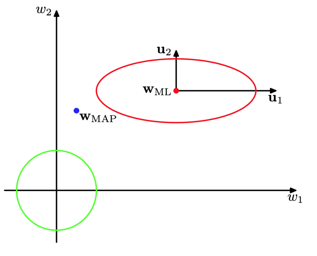
This means that the ratio $0 \le {\la_i \over \la_i + \alpha} \le 1$ measures the extent to which the data determine each parameter. Their sum, $\gamma \in [0, M]$ then measures the effective number of parameters estimated from the data.
We can use this observation to simplify our estimates of $\alpha$ and $\beta$ in the large data limit. In that limit, where $N \gg M$, the data should determine all the parameters, so $\gamma \to M$, and $\mm_N$ will tend to its maximum-likelihood value (which doesn’t contain $\alpha$). The estimate of $\alpha$ then simplifies to the precision of the of $\mm_N$, $$ {1 \over \alpha} = {2 E_W(\mm_N) \over M} = {1 \over M} \mm_N^T \mm_N,$$ and $\beta$ becomes the precision of the residuals,
$$ {1 \over \beta} = {2 E_D(\mm_N) \over N – M} \approx {2 E_D(\mm_N) \over N }= {1 \over N} \|\tt – \Phi \mm_N\|_2^2.$$
Discussion
What have we accomplished? We wanted a fully Bayesian approach to computing the predictive distribution for a new input. This required not only integrating over the model parameters but also the hyperparameters. Doing so was intractable, so instead we decided to replace the hyperparameters with their MAP estimates given the data. Assuming a flat prior on the hyperparameters, this amounted to maximizing their marginal likelihood. We derived an expression for the marginal likelihood for our Gaussian model and showed that, at least when the hyperparameters are known, we could use it to determine the number of parameters in our model. Of course, in our original setting, we don’t know the hyperparameters, so, for a given model order, we have to determine these by maximizing the marginal likelihood. We couldn’t do so in closed-form, so we resorted to an iterative method for computing them.
How well does our procedure perform? The figure below from Bishop shows an example where only $\alpha$ has to be estimated and indicates that using the estimate produces a nearly optimal test-error.
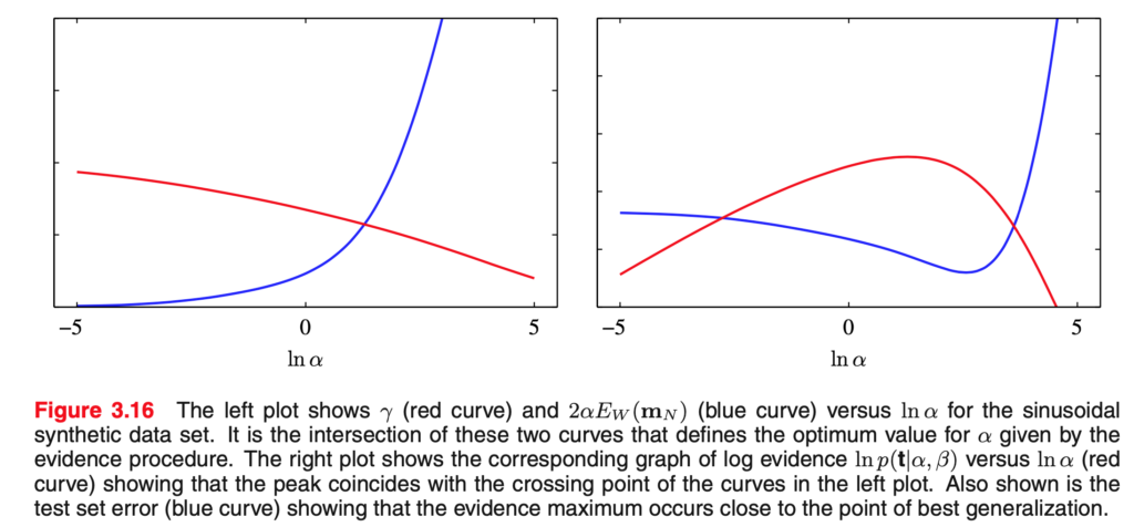
An important advantage of our approach is that $\alpha$ can be learned using the training data alone, whereas the usual procedure would require performing cross-validation or similar techniques to determine the optimal $\alpha$. This would be more computationally intensive, although it would by design yield the optimal generalization error.
And what about our original aim of computing the predictive distribution for a new input? Does our procedure produce a reasonable distribution? The nearly optimal generalization error is good, but it’s not technically what we were after. What we were after was an estimate of the predictive distribution for our model class. The generalization error tells us how well a point estimate from our model compares to the value drawn from the data distribution. So, it’s conceivable that we’d have a poor fit to the data distribution, but a good fit to our model’s predictive distribution.
However, assuming our model class is complex enough to capture the data distribution, then the predictive distribution should match the data distribution. In that case, what does good generalization error of our approximate distribution tell us?
The approximate distribution in the figure above is computed by setting $\beta$ to its true value $\beta^*$, and estimating $\alpha$ as $\hat \alpha$ using the procedure described here. Our approximate predictive distribution is then
$$ \hat p(t|\xx,\mathcal{D}) = \int p(t|\xx, \ww, \beta^*) p(\ww | \hat \alpha, \mathcal{D}) d\ww,$$ where $\mathcal{D} = (\tt, \XX)$ is the training data.
To compute RMS error we need to convert this to a point-estimate. Since RMS error involves the squared error, the point-estimate we want is the posterior mean: $$s(\xx) = \int t \, \hat p(t | \xx, \mathcal{D}) \, dt.$$
Instead of the RMS error, we’ll compute the mean squared error, as
$$ \text{MSE} = \EE_\xx \EE_{t \sim p^*(t|x)} (t – s(\xx))^2.$$ So we’re drawing inputs from their true distribution, drawing $t$ from the true conditional distribution given $\xx$, which we assume matches the predictive distribution, and then comparing to our estimate for that $\xx$.
Expanding this out, we get \begin{align}\text{MSE} &= \int d\xx \, p(\xx) \int p^*(t|\xx) \left(t\, – \int s\, \hat p(s|\xx) ds \right)^2 \, dt \\ &=\int d\xx \, p(\xx) \int p^*(t|\xx) (t^2\, – 2 t \overline{s} + \overline{s}^2) \, dt \\ &=\int d\xx \, p(\xx) (\overline{t^2}\, – 2 \overline{t} \overline{s} + \overline{s}^2) \\ &=\int d\xx \, p(\xx) (\overline{t^2}\, – \overline{t}^2 + \overline{t}^2- 2 \overline{t} \overline{s} + \overline{s}^2)\\ &=\text{var}(t|\xx) + \EE_\xx (\overline{t} – \overline{s})^2.\end{align}
The first term reflects the noise left in the predictions after the data has been accounted for, which we can’t do anything about. The second term is average squared difference between the posterior means of the true predictive distribution and our approximation. This is what we can adjust by changing the hyperparameters $\alpha$.
If we take the minimum generalization error in the figure above (the minimum of the blue curve) to reflect the noise variance, then the fact that the evidence approximation’s error is close to it means that the mean of the approximate posterior distribution is close, on average, to that of the true distribution.
That’s a useful fact to know about our estimator. However, it would have been useful to also consider the rest of the distribution. This could have been done in a toy, low-dimensional case, where we could compute the full integral needed for the predictive distribution directly, and compare the resulting distributions to those from the evidence approximation.
So, all-in-all, the evidence approximation allows us to estimate the full Bayesian predictive distribution by finding optimal hyperparameters using the training data alone, avoiding cross-validation. Estimators built on the approximate distribution have good generalization error in the example shown. It would have been useful to explore the performance of the approximation more thoroughly.
$$\blacksquare$$
Leave a Reply