Today I went back to trying to understand the solution when using the original regularization. While doing so it occurred to me that if I use a slightly different regularization, I can get a closed-form solution for the feedforward connectivity $Z$, and without most (though not all) of the problems I was having in my previous attempt at changing the regularizer.
Before describing the idea, let’s recall the connectivity decomposition. Our loss function is $$L(Z) = {1 \over 2 n^2} \|Y^T Y – X^T Z^T Z X \|_F^2 + {\lambda \over 2 m^2}\|Z – I\|_F^2.$$ As before, we apply SVD to write this as $$L(Z) = {1 \over 2 n^2} \|V_Y S_Y^2 V_Y^T – V_X S_X U_X^T Z^T Z U_X S_X V_X^T\|_F^2 + {\lambda \over 2 m^2}\|Z – I\|_F^2.$$ Letting $Q$ be an orthonormal completion of the basis formed by the columns of $U_X$, we can decompose the connectivity as \begin{align} Z &= U_X U_X^T Z U_X U_X^T + U_X U_X^T Z Q Q^T + Q Q^T Z U_X U_X^T + Q Q^T Z Q Q^T \\&= U_X \wt{Z}_{UU} U_X^T + U_X \wt{Z}_{UQ} Q^T + Q \wt{Z}_{Q U} U_X^T + Q \wt{Z}_{QQ}Q^T.\end{align}
We can then write the loss as \begin{align}L(Z) &= {1 \over 2 n^2} \|V_Y S_Y^2 V_Y^T – V_X S_X \wt Z_{UU}^T \wt Z_{UU} S_X V_X^T – V_X S_X \wt Z_{QU}^T \wt Z_{QU} S_X V_X^T\|_F^2\\ &+ {\lambda \over 2 m^2}\left(\|\wt{Z}_{UU} – I\|_F^2 + \|\wt{Z}_{QQ} – I\|_F^2 + \|\wt{Z}_{QU}\|_F^2 + \|\wt{Z}_{UQ}\|_F^2\right).\end{align}
The first term in the loss is the only thing keeping the regularization from sending $Z$ to $I$, and it only involves $\wt Z_{UU}$ and $\wt Z_{QU}$. Therefore, we know that regularization will set the remaining components to their regularization targets, and we can just consider the loss as a function of $\wt{Z}_{UU}$ and $\wt{Z}_{QU}$: \begin{align}L(\wt{Z}_{UU}, \wt{Z}_{QU}) &= {1 \over 2 n^2} \|V_Y S_Y^2 V_Y^T – V_X S_X (\wt Z_{UU}^T \wt Z_{UU} + \wt Z_{QU}^T \wt Z_{QU}) S_X V_X^T\|_F^2\\ &+ {\lambda \over 2 m^2}\left(\|\wt{Z}_{UU} – I\|_F^2 + \|\wt{Z}_{QU}\|_F^2\right).\end{align}
Notice how in the first term $\wt{Z}_{QU}$ shows up next to $S_X$, but in the regularization, it shows up alone. The idea is: since we have some freedom in choosing the regularization, why not regularize $\wt{Z}_{QU} S_X$ and $\wt{Z}_{UU} S_X$ instead?
In that case, the loss becomes \begin{align}L(\wt{Z}_{UU}, \wt{Z}_{QU}) &= {1 \over 2 n^2} \|V_Y S_Y^2 V_Y^T – V_X S_X (\wt Z_{UU}^T \wt Z_{UU} + \wt Z_{QU}^T \wt Z_{QU}) S_X V_X^T\|_F^2\\ &+ {\lambda \over 2 m^2}\left(\|\wt{Z}_{UU} S_X- I\|_F^2 + \|\wt{Z}_{QU} S_X\|_F^2\right).\end{align}
It’s then natural to define $$ F_U \triangleq \wt{Z}_{UU} S_X, \quad F_Q \triangleq \wt{Z}_{QU}S_X$$ in terms of which the loss is
\begin{align}L(F_U, F_Q) &= {1 \over 2 n^2} \|V_Y S_Y^2 V_Y^T – V_X F_U^T F_U V_X^T- V_X F_Q^T F_Q V_X^T\|_F^2\\& + {\lambda \over 2 m^2}\left(\|F_{U}- I\|_F^2 + \|F_{Q}\|_F^2\right).\end{align} Notice how $F_U$ and $F_Q$ have absorbed $S_X$ in the first term.
We can simplify further by defining stacking $$ F = \left[\begin{matrix}F_U \\ F_Q \end{matrix}\right], \quad F_0 =\left[\begin{matrix} I \\ 0 \end{matrix}\right]. $$ We then have the loss in terms of $F$ as \begin{align}L(F) &= {1 \over 2 n^2} \|V_Y S_Y^2 V_Y^T – V_X F^T F V_X^T\|_F^2 + {\lambda \over 2 m^2} \|F – F_0\|_F^2 \end{align}
Since the Frobenius norm is invariant to rotation, we can move $V_Y$ around in the first term. Defining $R = V_Y^T V_X$, we get, after shifting some constants to the regularizer $$L(F) = {1 \over 2} \|S_Y^2 – R F^T F R^T\|_F^2 + \la’ F^2, \quad \la’ \triangleq {\la n^2 \over 2 m^2}$$
Taking derivatives, \begin{align}\nabla_F L &= – 2 F (R^T (S_Y^2 – R F^T F R^T)R) + 2\lambda’ (F – F_0)\\
&=- 2 F (R^T S_Y^2 R – F^T F) + 2 \lambda’ (F – F_0).\end{align}
Setting this to zero and left-multiplying by $F^T$, we get
$$ F^T F (R^T S_Y^2 R – F^T F) = \lambda (F^T F – F^T F_0).$$
Left-multiplying by $(F^T F)^{-1}$ and rearranging $$ R^T \left(S_Y^2 – \lambda’ \right) R = F^T F- \lambda’ (F^TF)^{-1} F^T F_0.$$
Applying SVD $ F= U_F S_F V_F^T,$ and \begin{align} R^T \left(S_Y^2 – \la’ \right) R &= V_F S_F^2 V_F^T- \la’ V_F S_F^{-2} V_F^T V_F S_F U_F^T F_0\\ &= V_F S_F^2 V_F^T- \la’ V_F S_F^{-1} U_F^T F_0.\end{align}
The solution to this is to set $U_F^T = [V_F^T, 0].$ In that case $U_F^T F_0 = V_F^T$, and \begin{align} R^T \left(S_Y^2 – \la’\right) R &= V_F \left(S_F^2 – {\la’ \over S_F} \right) V_F^T,\end{align} so that $$ \boxed{V_F = R^T = V_X^T V_Y.}$$ The singular values $S_F$ are then the solutions to the independent cubic equations
$$\boxed{S_F^3 + \left(\la’ – S_Y^2\right)S_F – \la’ = 0.}$$ Checking the limits,
$$ \lim_{\lambda \to 0} S_F = S_Y, \quad \lim_{\lambda \to \infty} S_F = 1.$$
So we get $$ \boxed{F_U = V_F S_F V_F^T, \quad F_Q = 0}$$ with $V_F$ and $S_F$ as above, from which we get \begin{align}\boxed{\wt{Z}_{UU} = V_F S_F V_F^T S_X^{-1}, \quad \wt Z_{QU} = 0.}\end{align}
Remark: That was a lot of work to derive that $F_Q = 0$. If we knew that at the beginning we wouldn’t need the derivative of the loss and could just derive the expression for $F_U$ directly from it. I wonder if there’s a more direct way to see that $F_Q$ must be 0?
Translating this back to connectivity space,
\begin{align} Z &= U_X \wt{Z}_{UU} U_X^T\\ &= U_X V_F S_F V_F^T S_X^{-1} U_X^T \\ &= U_X V_X^T V_Y S_F V_Y^T V_X S_X^{-1} U_X^T.\end{align}
We can interpret this as
$$ Z = \underbrace{(U_X V_X^T)}_{\text{Nearest `rotation’ to } X} \cdot \underbrace{(V_Y S_F V_Y^T)}_{\text{Approximately } \sqrt{Y^T Y}} \cdot \underbrace{(V_X S_X^{-1}U_X^T)}_{\text{Left pseudoinverse of } X}$$
When applied to $X$, we get
$$ Z X = U_X V_X^T V_Y S_F V_Y^T V_X S_X^{-1} U_X^T U_X S_X V_X^T = U_X V_X^T V_Y S_F V_Y^T .$$
Finally, $$ X^T Z^T Z X = V_Y S_F V_Y^T V_X U_X^T U_X V_X^T V_Y S_F V_Y^T = V_Y S_F^2 V_Y^T.$$
This will tend to $Y^T Y$ at low regularization, and to the identity at high regularization. The latter makes sense in hindsight because our regularization is in the eigenspace of $U_X$, and the connectivity is such that the corresponding pseudounits produce unit variance at the output.
Numerical verification
Here is what an example $F$ matrix looks like for one of the fits:

So $F_Q$ is indeed zero, and $F_U$ is symmetric. I can then compare $V_F$ and $S_F$ to their predicted values:
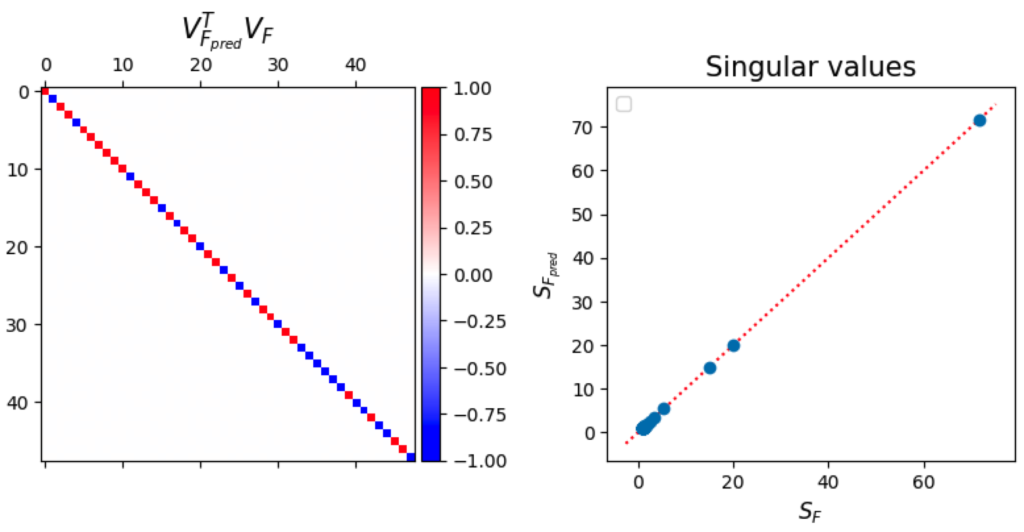
This shows a good match modulo the sign-flipping on the eigenvectors, which is unavoidable due to their inherent sign ambiguity.
So, the calculations seem correct.
$$\begin{flalign*} && \phantom{a} & \hfill \square \end{flalign*}$$
Leave a Reply