Linearizing the Covariance for the Free Model , Part III

As before, our loss in terms of deviations from the identity, is $$ L(\WW) = {1 \over 2} \|\SS – \XX^T (\II + \WW)^T \JJ (\II + \WW) \XX \|_F^2 + {\lambda \over 2} \|\WW\|_F^2.$$

Our linearization approach before was to consider a linearized version of this loss $\wt{L}(\WW)$, where we kept only the linear terms in $\WW$ inside the norm. That worked well except at one of the values, where there was a large discrepancy.

Here we’ll take a different approach, which uses the fact that we needed a lot of regularization. We’ll first work int terms of $\vareps = \lambda^{-1}$ and consider the equivalent loss $$ L(\WW) = {\vareps \over 2} \|\SS – \XX^T (\II + \WW)^T \JJ (\II + \WW) \XX \|_F^2 + {1 \over 2} \|\WW\|_F^2.$$

We can consider the full solution path $\WW(\vareps)$ indexed by the inverse regularization paramter $\vareps$. The solution at $\lambda = \infty$ corresponds to the solution at $\vareps=0$, where the likelihood term doesn’t contribute. So we get $\WW(0) = \bzero.$

The large values of regularization that we needed correspond to small values of $\vareps$. We can then approximate $$ \WW(\veps) \approx \WW(0) + \WW'(0) \veps = \WW'(0) \veps.$$

The gradient of the loss above is $$ \nabla L = \WW – 2 \vareps \JJ (\II + \WW) \XX \bE \XX^T,$$ where $\bE$ is the term in the norm. Setting the gradient to zero gives the implicit equation $$\WW = 2 \veps \JJ (\II + \WW) \XX \bE\XX^T,$$ implicit because $\bE$ is a function of $\WW$. Nevertheless, we can use it to evaluate the derivative, \begin{align*} \WW'(0) &= \lim_{\veps \to 0} \left. {\WW(\veps)- \WW(0) \over \veps}\right|_{\veps=0}\\ &= \left. 2 \JJ (\II + \WW) \XX \bE\XX^T\right|_{\WW=0}\\ &= 2 \JJ \XX (\SS – \XX^T \JJ \XX)\XX^T\\ &= 2 \XX (\SS – \XX^T \XX) \XX^T,\end{align*} where the last equality follows because $\JJ \XX = \XX$.

This then says that $$\WW(\veps) \approx 2 \XX (\SS – \XX^T \XX) \XX^T \veps .$$ Is that the case?

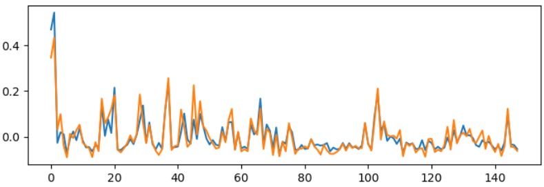
At high regularization ($\lambda=10^9$) there’s decent overlap, at least of the largest eigenvectors of the connectivity. In the figure below, blue is the first eigenvector of the learned connectivity, and orange is that of the estimate above.

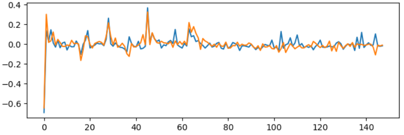
The match is similar at ($\lambda=10^6$). There’s also a good match for the second eigenvector,

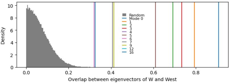
If we compare the overlaps of each pair of modes to what would be expected between two random vectors, several modes are aligned above chance:

So I think this is a sufficient first-order description of what’s going on.

$$\blacksquare$$