In the previous post we saw that linearzing the covariance for the Free connectivity model gives good results for high values of the regularization term $\lambda$, but not for the lower values which give the best validation error. At those values, the diagonal component of the weights starts becoming large. Below I’ve overlaid this diagonal component (orange) on the off-diagonal component (blue):
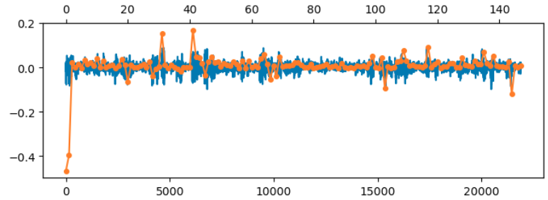
This suggests modeling the connectivity as $$\ZZ = \II + \WW + \DD.$$ We’ll assume that $\WW$ is small so that $\WW^T \WW \approx \bzero$. We will also ignore products of $\WW \DD$ for simplicity, but keep $\DD^2$.
Our loss is then \begin{align*} L(\WW) &= {1 \over 2} \|\SS – \XX^T (\II + \WW + \DD)^T \JJ (\II + \WW + \DD) \XX\|^2_F + {\lambda \over 2}\|\WW + \DD\|_F^2.\end{align*}
The inner term multiplying $\JJ$ expands to $$ \JJ + \JJ \WW + \JJ \DD + \WW^T \JJ + \WW^T \JJ \WW + \WW^T \JJ \DD + \DD^T \JJ + \DD^T \JJ \WW + \DD^T \JJ \DD.$$
If we assume that for typical elements of $\WW$ and $\DD$ that $ |W| < |D| < 1,$ then, in addition to $\WW^T \WW$, we can hope to ignore products of $\WW$ and $\DD$, $$ \approx \JJ + \JJ \WW + \JJ \DD + \WW^T \JJ + \DD^T \JJ + \DD^T \JJ \DD.$$
Let’s additionally approximate $\DD^T \JJ \DD$ by just $\DD^2$, to arrive at $$ \approx \JJ + \JJ \WW + \JJ \DD + \WW^T \JJ + \DD^T \JJ + \DD^2.$$
Then, using that $\JJ \XX = \XX$ for our centered data, and that $\WW$ will be symmetric at the optimum, we get $$ \XX^T (\dots) \XX \approx \XX^T \XX + 2 \XX^T \WW \XX + 2 \XX^T \DD \XX + \XX^T \DD^2 \XX.$$
Approximate our regularizer similarly, our approximate loss becomes $$ L(\WW, \DD) \approx {1 \over 2} \|\bE_0 – 2 \XX^T \WW \XX – 2 \XX^T \DD \XX – \XX^T \DD^2 \XX\|_F^2 + {\lambda \over 2}\|\WW\|_2^2 + {\lambda \over 2} \|\DD\|_F^2, \quad \bE_0 \triangleq \SS – \XX^T \XX. $$
At the optimium the gradient with respect to $\WW$ is then \begin{align*}\bzero = L_\WW &= -2\XX \bE \XX^T + \lambda \WW \\ &= – 2\XX (\bE_0 – 2 \XX^T \WW \XX – 2 \XX^T \DD \XX – \XX^T \DD^2 \XX)\XX^T + \lambda \WW \\ 2 \XX \bE_0 \XX^T – 2 \XX \XX^T (2 \DD + \DD^2) \XX \XX^T &= 4 \XX \XX^T \WW \XX \XX^T + \lambda \WW \\ 2 \XX \SS \XX^T – 2\XX \XX^T (\II + \DD)^2 \XX \XX^T &= 4\XX \XX^T \WW \XX \XX^T + \lambda \WW. \end{align*}
Decomposing $\XX = \UU \sqrt{\SS_X} \VV^T$ the above equation becomes $$ 2 \UU \sqrt{\SS_X} \VV^T \SS \VV \sqrt{\SS_X} \UU^T – 2 \UU \SS_X \UU^T (\II + \DD)^2 \UU \SS_X \UU^T = 4 \UU \SS_X \UU^T \WW \UU \SS_X \UU^T + \lambda \WW.$$
Multiplying the above equation on the left by $\UU^T$ and right by $\UU$, we get \begin{align} \label{main} \sqrt{\SS_X} \VV^T \SS \VV \sqrt{\SS_X} = \SS_X(\II + \DD)_{UU}^2 \SS_X + 2 \SS_X \WW_{UU} \SS_X + {\lambda \over 2}\WW_{UU},\end{align} which reduces to Eqn. 2 in our previous linearization attempt when $\DD = \bzero$.
For the gradient with respect to $\DD$, we’ll regroup terms in our loss and write it as $$ L(\DD) = {1 \over 2} \|\SS – 2 \XX^T \WW \XX -\XX^T (\II + \DD)^2 \XX \|_2^2 + {\lambda_D \over 2}\|\DD\|_2^2,$$ where we’ve generalized to allow $\DD$ its own regularizer.
The differential is then $$ dL = -\bE^T (4 \XX^T (\II + \DD) d\DD \XX) + \lambda_D \DD$$ from which we can read off the gradient as $$ L_D = -4 (\II + \DD) \XX \bE \XX^T + \lambda_D \DD,$$ where we’ve treated $\DD$ as a full matrix. The actual gradient would take the diagonal of this. Setting it to zero gives $$ [\XX \bE \XX^T] = {\lambda_D \over 4} {\DD \over \bone + \DD}.$$
The condition from the gradient on $\WW$ tells us that $2 \XX \bE \XX^T =\lambda \WW$. Substituting this in gives \begin{align*} 2 \lambda (\II + \DD) \WW &= \lambda_D \DD, \end{align*} which rearranges to $$ \DD = {2 \lambda \WW \over \lambda_D – 2\lambda \WW}.$$
In our standard regime above, $\lambda_D = \lambda$, so this simplifies to $$\DD = {2 \WW \over 1 – 2 \WW}.$$
This still couples $\DD$ to $\WW$ in a potentially awkward way. The Chatbots also pointed out that there’s an identifiability issue here with $\DD$ and $\WW$ overlapping on the diagonal, hence the coupling above.
An obvious way around this is to enforce $W_{ii}=0$. The standard way to do this is with Lagrange multipliers, but that will get messy. So instead we can try not regularizing $\DD$. In that case, it should mop-up the diagonal contribution of $\WW$, and $W_{ii}$ should go to zero through its own regularization.
With $\lambda_D = 0$, the gradient equation for $\DD$ becomes $$ -4(\II + \DD)\XX \bE \XX^T = -2\lambda (\II + \DD)\WW = 0 \implies (\II + \DD)\WW = 0,$$ which has two solutions: $D_{ii} = -1$, which incidentally is the limiting value when $\lambda_D \to 0$ above, or $W_{ii} = 0$, leaving $D_{ii}$ free. This latter is what we should get, given the regularization of $\WW$.
I went back to check the approximation in the $\lambda_D = \lambda$ case, where $ D_{ii} = 2 W_{ii}/(1 – 2 W_{ii}).$ We need to set the values of $\WW$ and $\DD$ from some learned $\ZZ$. Since $ \ZZ = \II + \WW + \DD,$ $$W_{i \neq j} = \ZZ_{ij}.$$ The on-diagonal terms satisfy $$ r_i \triangleq z_i – 1 = w_i + {2 w_i \over 1 – 2 w_i}.$$ Then $$ r_i (1 – 2 w_i) = w_i (1 – 2 w_i) + 2 w_i.$$
Rearranging, we get $$ 2 w_i^2 – (2 r_i +3 )w_i + r_i = 0.$$ We can solve this using the quadratic formula to get an expression for $w_i$. The negative root seems to give the right behaviour. Once we have an expression for $w_i$, we can use it to get one for $d_i$.
At that point $\WW$ and $\DD$ are completely specified, and we can plug them into Eqn. \ref{main} to see if it holds.
The fit seems OK, except for one large value where there’s a big discrepancy:
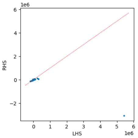
Those large values are precisely the ones we’re trying to capture…
$$\blacksquare$$
Leave a Reply