Below I’ve plotted the learned connectivity, minus the identity, for the Free model, which has no constraints. I used the regularization value, $10^6$, that gave the best validation $R^2$.
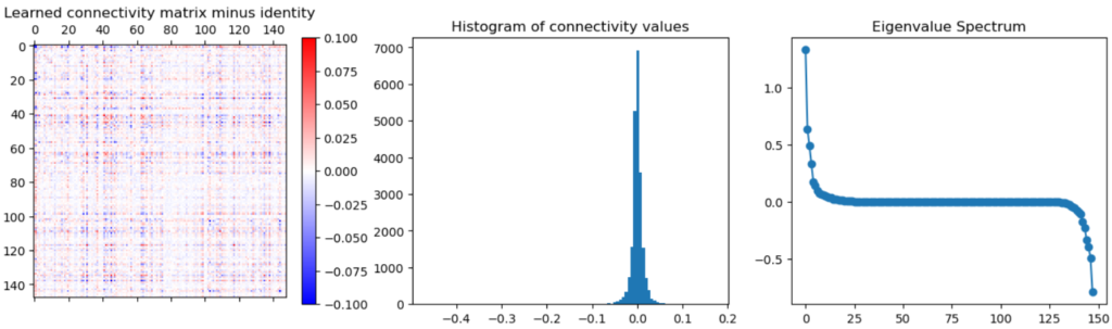
The connectivity deviations are indeed small, presumably because the regularization is so strong. Therefore linearization might be effective here as well.
Letting $\ZZ= \II +\WW$, our loss is \begin{align*} L(\WW) &= {1 \over 2} \|\SS – \XX^T (\II + \WW)^T \JJ (\II + \WW) \XX\|^2_F + {\lambda \over 2}\|\WW\|_F^2\\ &\approx {1 \over 2} \|\SS – \CC – \XX^T \WW^T \JJ \XX – \XX^T \JJ \WW \XX\|_F^2 + {\lambda \over 2}\|\WW\|_F^2\end{align*}
Then $$ dL = -\bE^T \XX^T d\WW^T \JJ \XX – \bE^T \XX^T \JJ d\WW \XX + \lambda \WW^T d\WW,$$ where we’ve defined $$\bE \triangleq \SS – \CC – \XX^T \WW^T \JJ \XX – \XX^T \JJ \WW \XX.$$
From which we read off the gradient as \begin{align} \nonumber \nabla L &= -2 \JJ \XX \bE^T \XX^T + \lambda \WW\\ \nonumber &= -2 \JJ \XX (\SS – \CC – \XX^T \WW^T \JJ \XX – \XX^T \JJ \WW \XX) \XX^T + \lambda \WW\\ &= – 2 \JJ \XX \bE_0 \XX^T + 2 \JJ \XX \XX^T \WW^T \JJ \XX \XX^T+ 2 \JJ \XX \XX^T \JJ \WW \XX \XX^T + \lambda \WW,\end{align} where we’ve defined the error at $\WW = \bzero$ as $$\bE_0 \triangleq \SS – \XX^T \XX.$$
Note the that the non-regularization part of this is symmetric. This means that the updates to $\WW$ will be symmetric, so its non-symmetric part will decay to zero, and the solution will be symmetric.
From the equation above we also have that \begin{align*} \bone^T \nabla L &= \bone^T 2 \JJ \XX \bE_0 \XX^T + 2 \JJ \XX \XX^T \WW^T \JJ \XX \XX^T+ 2 \JJ \XX \XX^T \JJ \WW \XX \XX^T + \lambda \bone^T \WW\\ &= \bzero + \bone^T \WW\\ &= \bzero \\ \implies \WW &= \JJ \WW.\end{align*}
We can then write the above gradient as $$ \nabla L =- 2 \JJ \XX \bE_0 \XX^T + 4 \JJ \XX \XX^T \WW \XX \XX^T + \lambda \WW.$$
Now $\XX$ is mean subtracted along the columns, so $\JJ \XX = \XX$, and the gradient becomes \begin{align*} \nabla L &=- 2 \XX \bE_0 \XX^T + 4 \XX \XX^T \WW \XX \XX^T + \lambda \WW \\ &= -2 \XX (\SS_Y – \XX^T \XX) \XX^T + 4 \XX \XX^T \WW \XX \XX^T + \lambda \WW \\ &= -2 \XX \SS_Y \XX^T + 2 \XX \XX^T \XX \XX^T + 4 \XX \XX^T \WW \XX \XX^T + \lambda \WW\end{align*}
Let $\XX = \UU \sqrt{\SS_X} \VV^T.$ In these terms, \begin{align*} \nabla L &= – 2 \UU \sqrt{\SS_X}\VV^T \SS_Y \VV \SS_X \UU^T + 2 \UU \SS_X^2 \UU^T + 4 \UU \SS_X \UU^T \WW \UU \SS_X \UU^T + \lambda \WW.\end{align*}
Multiplying on the left by $\UU^T$ and the right $\UU$, we get \begin{align*} \UU^T \nabla L \UU &= -2 \sqrt{\SS_X}\VV^T \SS_Y \VV \sqrt{\SS_X} + 2 \SS_X^2 + 4 \SS_X \WW_{UU} \SS_X + \lambda \WW_{UU} \end{align*}
Defining \begin{align*} \RR &\triangleq \VV^T \SS_Y \VV, \end{align*} we get \begin{align} \sqrt{\SS_X} (\RR – \SS_X) \sqrt{\SS_X} = 2 \SS_X \WW_{UU} \SS_X + {\lambda \over 2} \WW_{UU}. \end{align}
We can then solve for $\WW_{UU}$ element wise as \begin{align*} W_{UU, ij} &= {\sqrt{S_i}(R_{ij} – S_i \delta_{ij}) \sqrt{S_j} \over 2 S_i S_j + {\lambda \over 2} }\\ &= {R_{ij} – S_i \delta_{ij} \over 2 \sqrt{S_i S_j} + {\lambda \over 2 \sqrt{S_i S_j}} \delta_{ij}} \\ &={1 \over 2} {R_{ij} – S_i \delta_{ij} \over \sqrt{S_i S_j} + \lambda_{ij}}, \quad \lambda_{ij} \triangleq {\lambda \over 4 \sqrt{S_i S_j}}. \end{align*}
Trying it out
This works very well for high values of $\lambda$. The value that gives the best validation error is $10^6$. If we set $\lambda$ much higher, to $10^9$, then the approximation works very well. For example, we can return to equation 1, which equals zero at convergence. Moving the first term to the left hand side, we can plot its values against the right hand side:
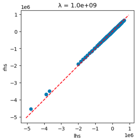
This shows a very good fit. However, at the value that gave the best validation error, the fit is not nearly as good:
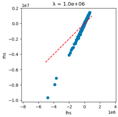
Below I’ve overlaid the diagonal values of $\WW$ in orange on the off-diagonal values in blue, on the same y-axis (the x-axes are different, since there are different numbers of elements). At the larger value of $\lambda$, the magnitudes are similarly small:
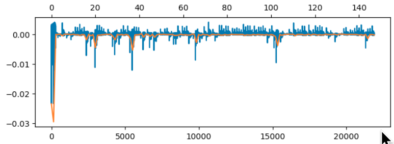
At the smaller, optimal value of $\lambda$, the magnitudes of some of the diagonal elements become large:
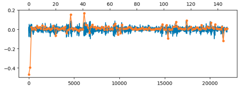
This indicates that we need to extend the model of the weights to include a diagonal component.
$$ \blacksquare$$
Leave a Reply