These are my running notes on Saxe et al.’s “A mathematical theory of semantic development in deep neural networks.” We are discussing this paper in the Discord sessions, so I will update these notes as we go.
Problem Setup
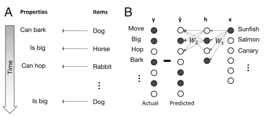
The learning problem they study is mapping items such as different plants and animals, to various properties, such as whether they can move, whether they are big, etc.
Their learning machine is a deep linear network. It’s deep because it has one hidden layer, and linear because the activations of all units are linear. Depth doesn’t add anything to the network’s input-output transformation, but, as it turns out, creates interesting learning dynamics.
They encode inputs $\xx$ are one-hot vectors indicating specific animals, plants etc. Target outputs are binary vectors $\yy$ indicating various properties of each input. Their predicted output is geneated by transforming the inputs to a hidden layer via a first set of weights $\WW_1$, and then transforming the hidden layer activations to predicted outputs $\hat \yy$ using a second set of weights $\WW_2$: $$ \hat \yy = \WW_2 \hh , \quad \hh = \WW_1 \xx.$$
Learning is performed by minimizing the least-squares loss $$L = {1 \over 2}\|\yy – \hat \yy\|_2^2.$$
Weight updates by gradient descent
Item-property pairs $(\xx_i, \yy_i)$ are presented in sequence. Weights are updated down the loss gradient after each such presentations. To find the gradients, we compute the differential $$ dL = -\bE^T d\WW_2 \WW_1 \xx – \bE^T \WW_2 d\WW_1 \xx,$$ where we’ve defined $$ \bE \triangleq (\yy – \hat \yy) = (\yy – \WW_2 \WW_1 \xx).$$
The gradients are then $${ \partial L \over \partial \WW_1} = -\WW_2^T \bE \xx^T = -\WW_2^T(\yy- \WW_2 \WW_1 \xx) \xx^T,$$ and $${\partial L \over \partial \WW_2} = -\bE \xx^T \WW_1^T = -(\yy – \WW_2 \WW_1 \xx) \xx^T \WW_1^T.$$
The weight updates are a stepsize $\lambda$ down these gradients: \begin{align*} \Delta \WW_1 &= -\lambda {\partial L \over \partial \WW_1} = -\lambda \WW_2^T(\yy- \WW_2 \WW_1 \xx) \xx^T \\ \Delta \WW_2 &= -\lambda {\partial L \over \partial \WW_2} = -\lambda (\yy- \WW_2 \WW_1 \xx) \xx^T \WW_1^T \end{align*}
From discrete to continuous time
To convert these discrete, per-item, updates into continuous time dynamics, we can take the changes above to occur over a time step $\Delta t$, and consider the net change after having viewed all $P$ items in the dataset.
For the first set of weights, this would look like \begin{align*} \Delta \WW_1 &= \Delta t \lambda \sum_{i=1}^P \WW_2^T(\yy_i- \WW_2 \WW_1 \xx_i) \xx_i^T\\ &= \Delta t \lambda \WW_2^T \left(\left(\sum_{i=1}^P \yy_i \xx_i^T\right)- \WW_2 \WW_1 \left(\sum_{i=1}^P \xx_i \xx_i^T\right)\right) \\ &= \Delta t \lambda P \WW_2^T (\Sigma_{yx} – \WW_2 \WW_1 \Sigma_x), \end{align*} where we’ve defined the covariances $$ {1 \over P} \sum_{i=1}^P \yy_i \xx_i^T = \Sigma_{yx}, \quad {1 \over P}\sum_{i=1}^P \xx_i \xx_i^T = \Sigma_x.$$
Then $$\lim_{\Delta t \to 0} {1 \over P \lambda}{ \Delta \WW_1 \over \Delta t} = \tau {d \WW_1 \over dt} = \WW_2^T (\Sigma_{yx} – \WW_2 \WW_1 \Sigma_x),$$ where we’ve defined $\tau \triangleq {1/P\lambda}$.
Similarly, for the second set of weights, we get $$ \tau {d \WW_2 \over dt} = (\Sigma_{yx} – \WW_2 \WW_1 \Sigma_x) \WW_1^T.$$
Weight dynamics
The dynamics above depend on both the input covariance $\Sigma_x$, and the input-output covariance $\Sigma_{xy}$.
First Simplification: Decorrelated Inputs
To gain insight into the weight dynamics, we can first simplify the problem by assuming that the input dimension are uncorrelated, so $ \Sigma_x = \II$.
We can then switch to coordinates that reflect the input and output statistics, by applying SVD to the input-output covariance, $$\Sigma_{yx} = \UU \SS \VV^T.$$
The columns of $\VV$ form an orthonormal basis for the input, and those of $\UU$ do the same for the output. Since the weights combine as $\WW_2 \WW_1$ to transform the inputs to the outputs, we can reparameterize the weights in terms of the $\UU$ and $\VV$ and an arbitrary orthogonal matrix $\RR$ as $$ \WW_1 = \RR \ol{\WW}_1 \VV^T, \quad \WW_2 = \UU \ol{\WW}_2 \RR^{T}.$$
We can express the dynamics in terms of this parameterization as \begin{align*} {d \WW_1 \over dt} &= \RR {d \ol{\WW_1} \over dt} \VV^T \\ \implies {d \ol \WW_1 \over dt} &= \RR^T {d \WW_1 \over dt} \VV\\ &= \RR^T\WW_2^T (\Sigma_{yx} – \WW_2 \WW_1 ) \VV \\ &= \RR^T \RR \ol{\WW}^T_2 \UU^T(\UU \SS \VV^T – \UU \ol{\WW}_2 \RR^T \RR \ol{\WW}_1\VV^T)\VV \\ &= \ol{\WW}_2 ^T( \SS – \ol{\WW}_2 \ol{\WW}_1). \end{align*}
Similarly, $$ {d \ol{\WW}_2 \over dt} = (\SS – \ol{\WW}_2 \ol{\WW}_1)\ol{\WW}_1^T.$$
Second Simplification: Diagonal Assumption
To further simplify the analysis, they now assume that $\ol{\WW}_1$ and $\ol{\WW}_2$ are diagonal, with elements $c_\alpha$ and $d_\alpha$ respectively. This makes the dynamics above decouple into \begin{align*} {d c_\alpha \over dt} &= (s_\alpha – c_\alpha d_\alpha) d_\alpha \\ {d d_\alpha \over dt} &= (s_\alpha – c_\alpha d_\alpha) c_\alpha \end{align*}
The dynamics of the net transformation $\WW_2 \WW_1$ in the transformed coordinates are then captured by the dynamics of the product $\ol{\WW}_2 \ol{\WW}_1$, which, under our diagonal assumption, reduce to the dynamics of $a_\alpha = c_\alpha d_\alpha$: $$ {d a_\alpha \over dt} = {d c_\alpha \over dt} d_\alpha + c_\alpha {d d_\alpha \over dt} = (s_\alpha – c_\alpha d_\alpha)( c_\alpha^2 + d_\alpha^2).$$
Third Simplification: Balanced Regime
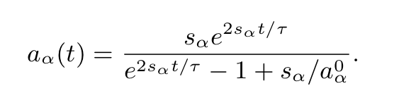
They then simplify further and study the balanced regime where $c_\alpha = d_\alpha$, which yields $$ {d a_\alpha \over dt} = 2 a_\alpha (s_\alpha – a_\alpha) .$$
Solving this ODE for the final value of $a_\alpha$ and assuming an integration time constant $\tau$ (we used 1 above for clarity) gives the sigmoidal dynamics in the main text,
$$ \blacksquare$$
Leave a Reply