We’re after insight, not an exact solution. ChatGPT had a good suggestion to linearize the loss around $\zz = 1$. The empirical values we see for $\zz$ can be quite large relative to 1, in the range $[-0.5, 1.5]$, but linearization might be enough to give the insight we’re after. Let’s see.
If we consider $\bdelta = \zz – \bone$, then $$L(\bdelta) = {1\over 2}\|\XX^T[\bdelta + \bone]^2 \JJ [\bdelta + \bone] \XX – \SS\|_2^2 + {\lambda \over 2}\|\bdelta\|_2^2.$$
We can linearize the middle as \begin{align*} [\bdelta + \bone]\JJ[\bdelta + \bone] &= [\bdelta] \JJ + \JJ [\bdelta] + \JJ \end{align*}
When we left and right multiply by $\XX^T$, each of these contributes a term.
The first is $$ \XX^T [\bdelta] \JJ \XX = \sum_i \delta_i \xx_i \widetilde \xx_i^T,$$ where $\widetilde \xx_i$ are the population-mean-subtracted (i.e. per-odour) responses. So it’s not that each $\xx_i$ will have mean zero.
The second is $$ \XX^T \JJ [\bdelta] \XX = \sum_i \delta_i \widetilde \xx_i \xx_i^T.$$
We can combine these into a single term $$ \sum_i \GG_i \delta_i, \quad \GG_i \triangleq \xx_i \widetilde \xx_i^T + \widetilde \xx_i \xx_i^T.$$
We can combine the last term with the target covariance using $$ \SS – \XX^T \JJ \XX \triangleq \bE_0,$$ where the subscript reminds us that this is the error at $\bdelta = 0.$
If we vectorize, forming $$\GG = [\bg_1 \dots \bg_N], \quad \bg_i = \text{vec}(\GG_i),$$ and similarly for the other terms, our loss will be $$ L(\bdelta) = {1 \over 2} \|\GG \bdelta – \ee_0\|_2^2 + {\lambda \over 2} \|\bdelta\|_2^2.$$ The gradient is then $$ \nabla L = \GG^T (\GG \bdelta – \ee_0) + \lambda \bdelta,$$ so the solution is $$ \boxed{\bdelta = (\GG^T \GG +\lambda \II) ^{-1} \GG^T \ee_0.}$$
If we ignore correlations among the $\bg_i$, this is $$ \delta_i \approx {\bg_i^T \ee_0 \over \|\bg_i\|_2^2 + \lambda}.$$
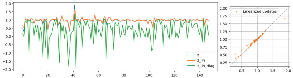
The linear update is good (orange)! However, the correlations among the columns of $\GG$ are important, since ignoring them, and just taking the variances, clearly produces a poor estimate.
Explanations
Now, how to intuitively explain the linear approximation?
One idea I had was to see whether there was an equivalent dataset, one that would give the same coefficients, for the the same $\ee_0$, but would have decorrelated representational atoms $\bg_i$, so that the explanation that ignored those correlations would work, and we could explain the results that way.
However, no such dataset exists. Let $\GG = \UU \SS \VV^T$. Then $$ (\GG^T \GG + \lambda \II)^{-1} \GG^T = \VV {\SS \over \SS^2 + \lambda \II} \UU^T.$$ There are no degrees of freedom here, that would allow us to e.g. rotate $\VV$ – once $\GG$ is known, everything is determined.
Another possibility is to switch coordinates: rearrange the above to get multiply both sides on the left by $\VV^T$, and we get $$ \UU^T \ee_0 = \left[{\SS \over \SS^2 + \lambda \II}\right]^{-1} \VV^T \bdelta.$$ This has the disadvantage that we’re no longer explaining the gains $\bdelta$ themselves, but some rotated version.
A further possibility is to simply define the raw overlaps as $\GG^T \ee_0$, and take the rows of $(\GG^T \GG + \lambda \II)^{-1}$ as the cell-specific filters.
ChatGPT suggested an improvement on this, where we split the filters into two whitening steps $$ (\GG^T \GG + \lambda \II)^{-1} \triangleq \WW^2, \quad \WW = (\GG^T \GG + \lambda \II)^{-{1 \over 2}}.$$ We can then write $$ \delta_i = \ee_i^T \WW \WW (\GG^T \ee_0) = \langle \WW \ee_i, \WW (\GG^T \ee_0) \rangle.$$
If there were no correlations, $\delta_i \propto \ee_i^T \GG^T \ee_0.$ With the correlations, we have to whiten both the filter $\ee_i$, and the overlaps, $\GG^T \ee_0,$ which is what we have above.
I think that’s the best we can do.
$$ \blacksquare$$
Leave a Reply