At lab meeting today we discussed a paper showing that mice use stereo-olfaction to determine their head-direction. A few key panels are below:
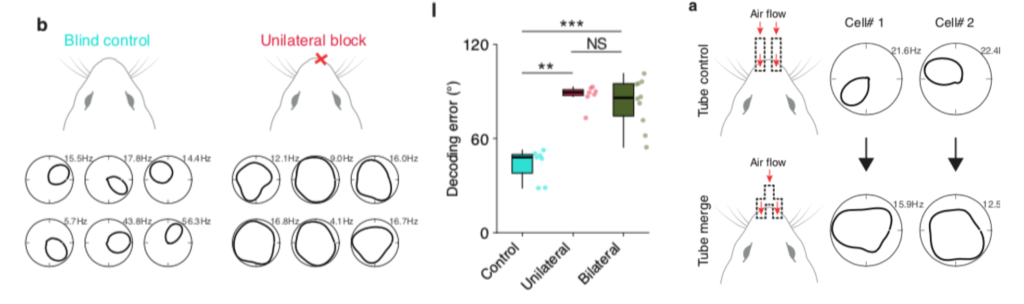
The first one shows the tuning of some head-direction cells in control mice. These mice were blind so had to use other modalities, to compute head direction. Indeed, when one of the nostrils was blocked, the head-direction tuning mostly disappeared. Decoding of head-direction was correspondingly perturbed, as shown in the middle panel. If the mice weren’t using olfactory cues, then blocking the nostril shouldn’t have made a difference. If they were using mono-olfaction, then blocking a single nostril also shouldn’t have made a difference. Further, they found that if they presented the same odour stream to both nostrils, head-direction was similarly perturbed.
These findings are consistent with the mice using stereo-olfaction as a cue for computing head-direction. The question is why they seem to use the differential signal provided by the two nostrils, presumably signalling spatial concentration gradients, rather than the common signal that would signal raw concentration. Is there more information in the differential signal?
Is there more information in concentration gradients?
To address this question we can consider the situation of a mouse facing upwind toward an odour source:
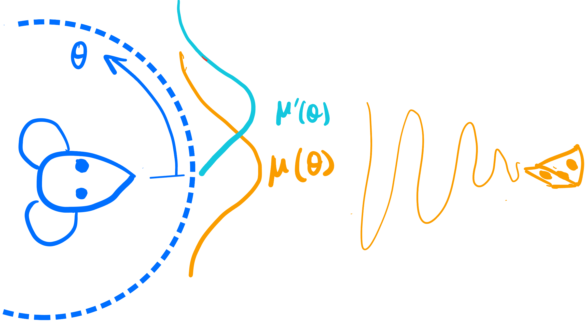
As the mouse rotates its head, the odour concentration at its snout will change (orange curve above). We can then determine how informative this changing concentration profile is about the angle of the mouse’s head. This would correspond to the mono-olfaction case. We can model the stereo-olfaction case as sensitivity not to the raw concentration itself, but its spatial derivative (the blue curve above).
To simplify the problem we’ll assume that the odour concentation profile is Gaussian in head-angle. So the mean concentration as a function of head angle is $$ \mu(\theta) = c_0 e^{-\theta^2/2},$$ where $c_0$ is the maximum concentration.
Mono-olfaction
We’ll need a model of how this mean concentration determines the flucutating signal at a nostril. Perhaps the simplest model is to imagine the mean concentration as the average rate of arrival of odour packets from the source. If we assume these odour packet arrivals are memoryless, then the corresponding model is a Poisson process with rate determined by the concentration. We’ll assume that the odour packets are arriving fast enough that we can approximate the Poisson process with a Gaussian with the same mean and variance. So our mono-olfaction signal would be $$ m(\theta) \sim \text{Poisson}(\mu(\theta)) \approx \mathcal{N}(\mu(\theta), \mu(\theta)).$$
We can define a corresponding SNR as the ratio of the mean to the standard deviation: $$ \text{SNR}_1 = {\mu(\theta) \over \sqrt{\mu(\theta)}} = \sqrt{\mu(\theta)}.$$
Stereo-olfaction
It will be useful to think of the mono-olfaction signal as a mean signal plus some Gaussian noise $\eta$ with variance $\mu(\theta)$: $$ m(\theta) = \mu(\theta) + \eta, \quad \eta \sim \mathcal{N}(0, \mu(\theta)).$$
The stereo-olfaction signal would be similar, but with two channels, $s_1$ and $s_2$. Let’s assume that the two nostrils are at an angle of $\pm \Delta \theta/2$ relative to the head direction. The signal at the first nostril would then be $$ s_1(\theta) = \mu\left(\theta – {\Delta \theta \over 2}\right) + \eta_1, \quad \eta_1 \sim \mathcal{N}\left(0, \mu\left(\theta – {\Delta \theta \over 2}\right)\right).$$
If we assume that the inter-nostril distance is small compared to the length scale over which concentrations change, we can approximate this as $$s_1(\theta) \approx \mu(\theta) – \mu'(\theta) {\Delta \over 2} + \eta_1, \quad \eta_1 \sim \mathcal{N}(0, \mu(\theta)).$$
The signal at the second would be similar, but at the angle of the second nostril, $$ s_2(\theta) \approx \mu(\theta) + \mu'(\theta){\Delta \over 2} + \eta_2, \quad \eta_2 \sim \mathcal{N}(0, \mu(\theta)).$$
The signal at the second would be similar to the first, but sensing the concentration at a slightly shifted angle, determined by the inter-nostril distance: $$s_2(\theta) = \mu\left(\theta + \Delta \theta\right) + \eta_2, \quad \eta_2 \sim \mathcal{N}(0, \mu(\theta + \Delta \theta)).$$
A key point is that the noise at the second nostril is correlated with the noise at the first by the length scales of the plume at the nose. Letting this correlation be $\rho$, we have $$\eta_2 = \rho \eta_1 + \sqrt{1 – \rho^2} \eta, \quad \eta \sim \mathcal{N}(0, \mu(\theta)),$$ where $\eta$ is the noise component at the second nostril that’s uncorrelated with that at the first.
The stereo difference
What should we do with the two stereo signals? Adding them basically reproduces the mono-signal, with slightly reduce noise.
The natural thing to do is to subtract the signals. This gives the stereo difference: \begin{align*} \Delta s(\theta) &= s_2(\theta) – s_1(\theta)\\ &=\mu'(\theta) \Delta \theta + \eta_s,\end{align*} where $\eta_s$ is the noise term, $$ \eta_s = – (1 – \rho)\eta_1 + \sqrt{1 – \rho^2} \eta.$$
The two noise components $\eta_1$ and $\eta$ are uncorrelated so their variances add: \begin{align*} \text{var}(\eta_s) &= (1 – \rho)^2 \var(\eta_1) + (1 – \rho^2) \var(\eta)\\ &= (1 – 2 \rho + \rho^2 + 1 – \rho^2) \var(\eta_1) \\ &= 2 (1 – \rho)\mu(\theta). \end{align*}
Correlations start at 1 when the inter-nostril distance as 0 and decay as the distance increases. The decay rate we saw in our 2D simulations was exponential, but Gaussian decay makes the math a little cleaner. If we assume that this decay is Gaussian, we can write $$ \rho = e^{-\Delta \theta^2 / 2 L} \approx 1 – {\Delta \theta^2 \over 2 L}, $$ where $L$ is the relevant correlation length scale of the air. Therefore $$\var(\eta_s) \approx {\Delta \theta^2 \over L^2} \mu(\theta).$$
Therefore, our stereo difference behaves as $$ \Delta s(\theta) \approx \mu'(\theta) \Delta \theta + \eta_s, \quad \eta_s \sim \mathcal{N}\left(0, {\Delta \theta^2 \over L^2} \mu(\theta)\right).$$
We can then define a stereo SNR as the ratio of the mean magnitude to the standard deviation, $$ \text{SNR}_2 = {|\mu'(\theta)| \Delta \theta \over \sqrt{{\Delta \theta^2 \over L^2} \mu(\theta)}} = {|\mu'(\theta)| L \over \sqrt{\mu(\theta)}}.$$
When to turn on the stereo
We can determine the relative advantage of stereo to mono olfaction as the ratio of the SNRs: $$ \boxed{ {\text{SNR}_2 \over \text{SNR}_1} = { {|\mu'(\theta)| L \over \sqrt{\mu(\theta)}} \over \sqrt{\mu(\theta)}} = { |\mu'(\theta)| L \over \mu(\theta)}.}$$
For our Gaussian plume this simplifies further: $$ \mu(\theta) = c_0 e^{-\theta^2/2} \implies \mu'(\theta) = – c_0 \theta e^{-\theta^2/2} = -\theta \mu(\theta).$$ We then get $$ {\text{SNR}_2 \over \text{SNR}_1} = \theta L.$$
Summary
What the expression above says is that stereo olfaction is useful when at the edges of the plume (where $\theta$ is larger), or other places where the concentration changes rapidly (odour edges). This sensitivity to concentration changes is a natural consequence of the stereo signal being the difference of the signals from the two nostrils.
The advantage of stereo olfaction is magnified when the spatial length scale of correlations in the fluid is large, like the laminar boundary-layer flow near the ground where the mice are. This ensures that the noise at the two nostrils is sufficiently correlated that subtracting the two (mostly) cancels out the noise.
In short, stereo-olfaction is best when you’re searching surfaces for olfactory edges!
$$ \blacksquare$$
Leave a Reply