Activity-Dependent Synchronization of Linear Integrate and Fire Units

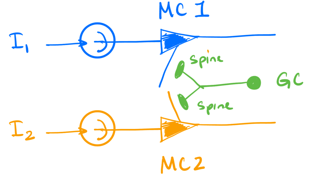
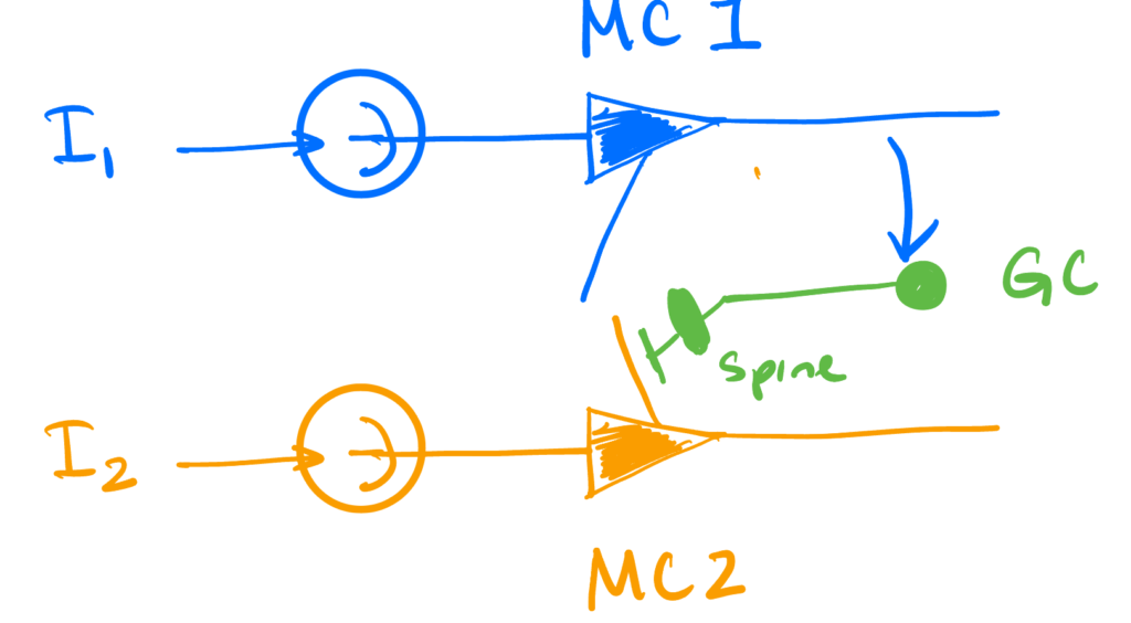
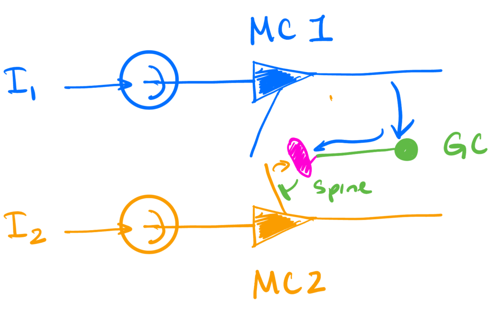
We’re interested in activity-dependent synchronization. This is where the inhibition that a mitral cell receives from a granule cell spine requires that spine to have been previously depolarized enough to activate the NMDA channels that are required (via both the additional depolarization of the spine and increased Ca2+ influx they provide) to cause vesicle release.

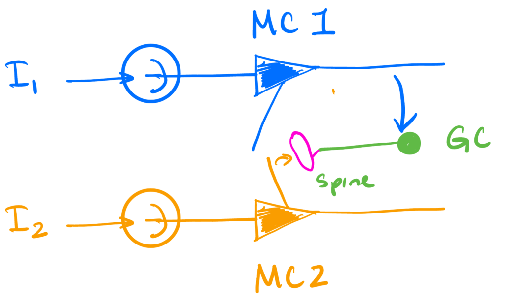
We will model this with just two mitral cells and one granule cell connecting the two. The dynamics below will focus on the mitral cells. The granule cell itself will be invisible, its only role being the physical implementation of the inhibition we will introduce.

Spiking introduces discreteness into the dynamics, which complicates the analysis. So we’ll build things up in stages:

1. We’ll start with a single neuron firing to constant current input.
2. We’ll then add (vanilla) self-inhibition.
3. We’ll then connect the neurons. Before trying the activity-dependent self-inhibition, we’ll practice on feed-forward inhibition: whenever the first neuron spikes, it will inhibit the other, but not vise-versa.
   • This will also serve as a good “control” case for synchronization.
4. We’ll then bring self-inhibition back for the second neuron, but have it require the granule cell delivering the inhibition to have been primed by a recent spike from the first neuron.
5. Finally, we will enable these activity dependent self-inhibitions for both neurons.

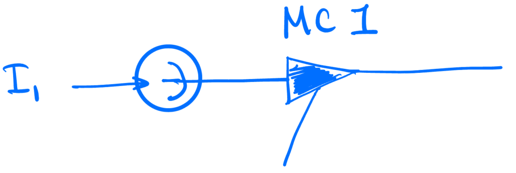
1. One neuron

We’ll start with a single unit. Its dynamics will be simply $$ \dot v = I, \quad v(t) = 1 \implies v(t^+) \leftarrow 0.$$ So it integrates the current $I$ until its voltage reaches 1, at which point its voltage is reset to 0.

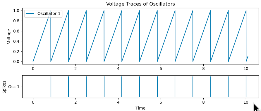
The time between spikes is simple integration. So valid solutions to the dynamics above will consist of such integration intervals, each ending in a spike.

We can think of this as a partitioning of the time line into semi-open intervals $(t_i, s_{i}], (t_{i+1},s_{i+1}], \dots.$ We’ve used $t$ and $s$ to indicate the start and end of an interval, so $t_{i+1} = s_{i}^+.$ Since each interval ends in a spike, the spike times are given by the $s_i$.

Inside each interval, we have \begin{align*} v(t) &= v(t_i) + I(t – t_i) \\ v(t_i) &= 0 \quad \text{(reset condition)}\\ v(s_i) &=1 \quad \text{(spiking condition)}. \end{align*} Combining all these gives $$s_i – t_i = {1 \over I}.$$ This tells us that our solutions partition the timeline into equal sized intervals of size $1/I$ i.e. regular firing, as expected.

2. Self-Inhibition

Next we’ll add self-inhibition. This is to model a mitral cell exciting a granule cell spine, which immediately applies some inhibition back onto the mitral cell.

The only update to our dynamics above is that $$ v(t) = 1\implies v(t^+) = -\Delta,$$ where $\Delta$ is the strength of the inhibition.

The effect of this inhibition should be to reduce the frequency of the regular spikes. Inside any solution interval, we now have \begin{align*} v(t_i) &= -\Delta \\ v(s_i) &= 1 = v(t_i) + I (s_i – t_i), \end{align*} so $$ s_i – t_i = {1 + \Delta \over I}.$$ So the periods do indeed increase by the additional amount needed to overcome the inhibition.

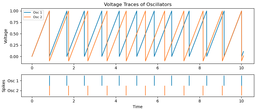
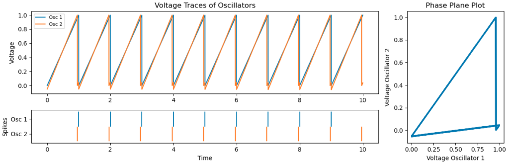
Below we’ve added a new neuron (orange) with self-inhibition to compare to the one without, and indeed observe regular firing at a lower frequency.

3. Feed-forward inhibition

In this setting, we have two neurons. The first will inhibit the second by an amount $\Delta$ whenever it spikes. So our dynamics are \begin{align*} \dot \vv &= \II\\v_1(t) &=1 \implies \begin{aligned}[t] v_1(t^+) &\leftarrow 0\\ v_2(t^+) & \leftarrow v_2(t) – \Delta \quad (\text{Feed-forward inhibition})\end{aligned}\\v_2(t) &= 1 \implies v_2(t^+) \leftarrow 0. \end{align*}

These dynamics are easiest to understand when we plot in the $(v_1, v_2)$ phase space:

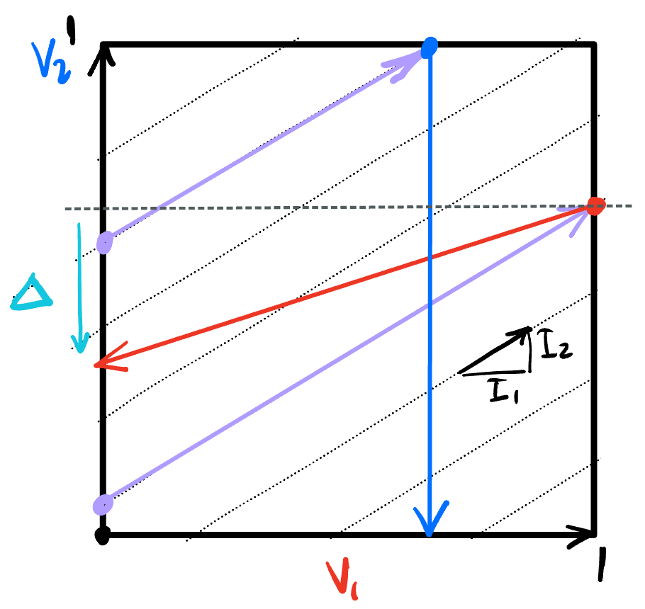
Starting at any point inside the space, integration moves along the dashed lines. A couple such trajectories are shown in purple. When such a trajectory hits the right boundary, such as at the red point, $v_1 = 1$, so that variable resets to 0, shifting the point to the left boundary. If $v_2$ kept its value, the phase point would be moved horizontally, along the dashed line. However, the feedforward inhibition means $v_2$ is reduced by $\Delta$, and the reset is to the end point of the red arrow.

On the other hand, when the trajectory hits the top boundary, $v_2 = 1$, so that voltage is rest, transporting the point vertically down, since the voltage on $v_1$ is maintained.

The dynamics bounce around in this way inside the phase box, generating spikes whenever they hit the boundary.

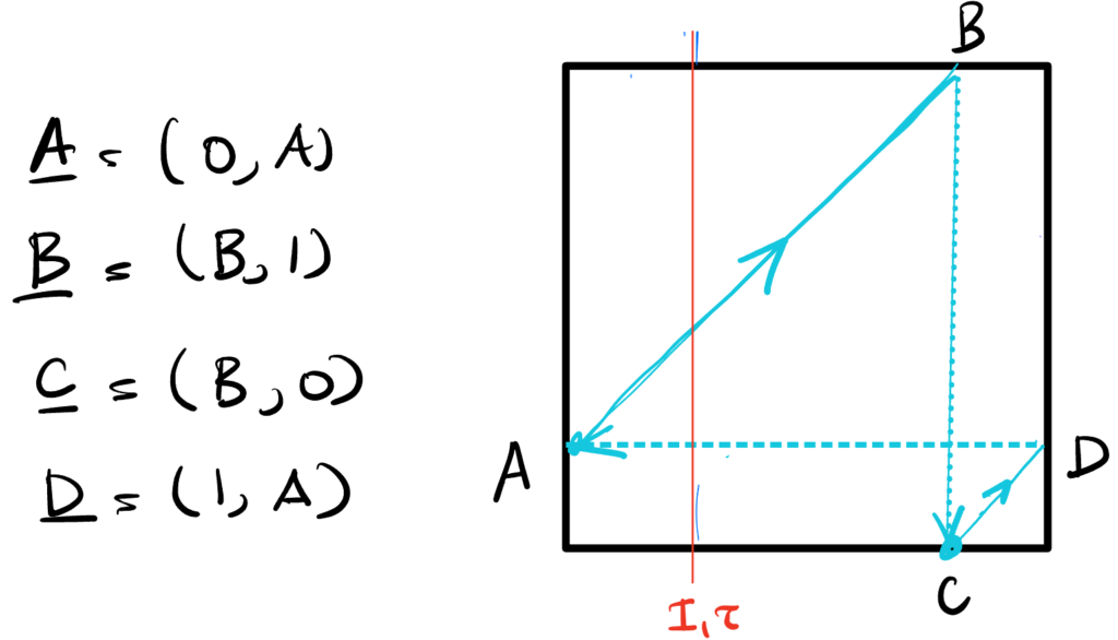
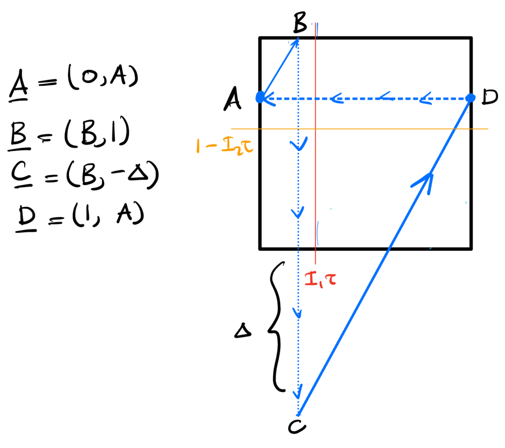
We’re after synchronous dynamics. These dynamics should be cyclical, and generate one spike each per cycle. Therefore, they should look something like,

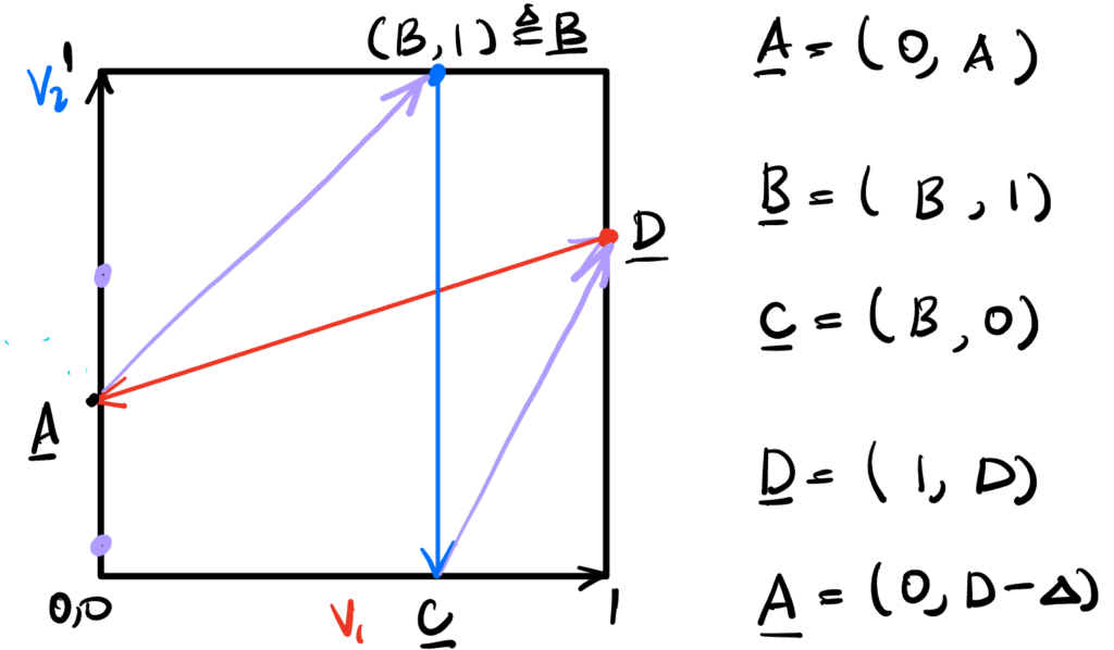
with the only caveat that the slopes of the trajectories inside the phase space (the purple arrows) should be the same, $I_2/I_1$. We use this fact to determine solutions.

First, the trajectory from A to B: the rise is $1 – A$ and the run is $B$, so $${1 – A \over B} = {I_2 \over I_1} \implies B = (1 – A){I_1 \over I_2}.$$

Next, the trajectory from C to D: the rise is $D$ and the run is $1 – B$, so $${I_2 \over I_1} = {D \over 1 – B} \implies B = 1 – D{I_1 \over I_2}.$$

Since $A = D – \Delta$, equating the last two expressions for $B$ gives $$ (1 – D + \Delta){I_1 \over I_2} = 1 – D{I_1 \over I_2},$$ from which we can solve for the magnitude of the inhibition $$\boxed{\Delta = {I_2 \over I_1} – 1 \ge 0.}$$

This makes sense: the second unit is the one getting inhibited, so its driving current, $I_2$, must be larger than that of the other unit. Synchrony occurs when the phase delay induced in the second unit by the inhibition exactly compensates for the additional drive it receives. Letting $T_1$ and $T_2$ be the periods of the two oscillators, we can derive an expression for the inhibition by equating theses two $$T_2 = {1 + \Delta \over I_2} = {1 \over I_1} = T_2 \implies \Delta = {I_2 \over I_1} – 1.$$

Below is an example for $I_2/I_1 = 1.1$, and $A = -\Delta/2$:

From the above it looks like we have one free parameter. Let’s make sure that all the parameters are in the valid range.

Let’s take $A$ to be the free parameter. We have that $B = (1 – A){I_1 \over I_2}.$ We know that $A \le 1$, so $B \ge 0$. For $B \le 1$, we need $A \ge 1 – {I_2 \over I_1} = -\Delta.$

What happens if $A < -\Delta$? In that case, it takes a few cycles to lock in to the synchronization. Let $A[0]$ be that initial value of $A$. A time $1/I_1$ later, unit 1 will spike. The voltage of unit 2 at that point will be $A[0] + {I_2 \over I_1} < 1$, so unit 2 won’t have spiked in that time, and will receive inhibition. We then have $$A[n+1] = A[n] + {I_2 \over I_1} – \Delta = A[n] + 1.$$

So the post-reset voltage of unit 2 will increase by 1, until it’s in the range $$ -\Delta \le A \le 1.$$ This range is larger than 1, so there is no chance that the reset voltage won’t eventually fall into it. Therefore, the dynamics are attractive for $A < -\Delta.$

Comments

• We need the inhibition $\Delta$ to be set to the correct value.
• What matters is the ratio of currents to the two units – this builds in an invariance.
  • If the currents are directly proportional to the odour concentration, this gives concentration invariance.
• The time from when unit 2 spikes to when unit 1 spikes is $$ {1 – B \over I_1} = D = A + \Delta.$$ The threshold is fixed by the current ratio, so what this says is that the initial condition, $A$, is encoded in the spike phases. It also shows that a whole family of solutions exist. This isn’t surprising because our system is mostly linear, so won’t exhibit limit cycles.
  • Ideally, we wouldn’t want such dependence on the initial condition. The spike phases should be determined purely by the currents, not by initial conditions.

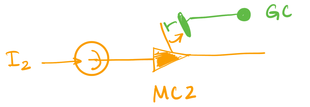
4. Activation-Dependent Self Inhibition

In this setting, we will have the second neuron provide self-inhibition, but will require the GC providing this inhibition to have been recently activated by the first unit. The first unit will be without self-inhibition.

So the dynamics will be \begin{align*} \dot v &= \II \\ v_1(t) &= 1 \implies \begin{aligned}[t] v_1(t_+) & = 0 \\ t_1 & \leftarrow t \quad &\text{ (spine activation time)}\end{aligned}\\ s(t) &= 1 – \Theta(t – t_1 – \tau) \quad \quad \quad \quad \quad \quad \text{(spine deactivates after $t_1 + \tau$)}\\ v_2(t) &=1 \implies v_2(t_+) = – s(t) \Delta \quad \text{(self-inhibition if spine is active)} \end{align*}

In this setting we have two pictures.

4.1 Inactive spine

When the time between when the first neuron spikes and when the second spikes is too long, the granule cell spine is deactivated, and no self inhibition of the second neuron occurs.

The spine deactivates after a time $\tau$, which corresponds to a change in voltage of $I_1 \tau$ in the first unit. So the phase picture we have is

The only setting in which this configuration has synchronous solutions is when $I_1 = I_2$. We can see this by going around the loop.

Going from $A$ to $B$, we have $$ { 1- A \over B} = {I_2 \over I_1} \implies B = (1 – A){I_1 \over I_2}.$$

Going from $C$ to $D$, we have $${D \over 1 – C} = {A \over 1 – B} = {I_2 \over I_1} \implies 1- B = {I_1 \over I_2} A \implies B = 1 – {I_1 \over I_2} A.$$ Equating the last two equations gives $$ {I_2 \over I_1} = 1.$$

So this configuration is a solution only when the two input currents are the same. When that’s the case, then any $B = (1 – A) > I_1 \tau$ will be a solution:

4.2 Active spine

This is the more interesting case, and will occur when $B < I_1 \tau$. In that case, the second neuron receives self-inhibition of amount $\Delta$ when it spikes.

The phase picture is:

We can again go around the loop. As before, $A$-to-$B$ gives $$ B = {I_1 \over I_2} (1 – A).$$ This time, $C$-to-$D$ gives something different, $${A + \Delta \over 1 – B} = {I_2 \over I_1} \implies A + \Delta = {I_2 \over I_1}(1 – B) = {I_2 \over I_1}\left(1 – {I_1 \over I_2}(1 – A)\right),$$ from which we get $$A + \Delta = {I_2 \over I_1} – 1 + A \implies \Delta = {I_2 \over I_1} – 1.$$

The spine being active requires $$B < \tau I_1 \implies {I_1 \over I_2}(1 – A) < \tau I_1 \implies (1 – A) < \tau I_2 \implies A > 1 – \tau I_2.$$

So, for a given set of current, if we set the threshold correctly, and start $A$ large enough, we should get a synchronous solution.

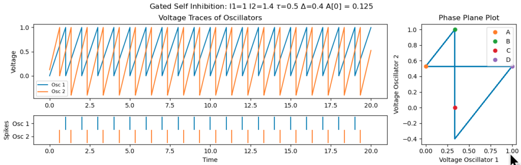
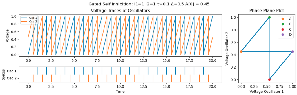
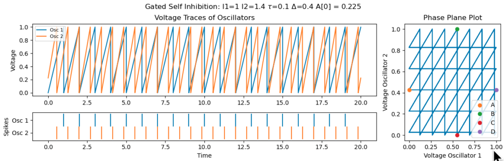
It’s important that $\tau$, the activation duration of the spine, is large enough. Otherwise, poor initializations can leave the system stuck in non-synchronous regime. The example below is for the same initial conditions as above, but with $\tau$ set to 0.1, instead of 0.5, requires the first neuron to firing within 0.1 of the second for the second to experience self-inhibition:

Summary

We’ve taken a loose definition of synchronization here as cyclic activity that generates one spike per neuron per cycle. We’ve found that:

• Without inhibition, synchronization can only occur if the two neurons receive the same current.
• With inhibition, synchronization can occur over a range of current drives. But it requires that the inhibition be onto the more driven unit, and compensate the additional drive it receives.
• Because of this compensation requirement, the size of the synchronizing inhibition depends on the relative currents the two units receive.
• Exactly when the second unit receives the inhibition doesn’t matter. So it can be as feed-forward inhibition from the first unit, or as self-inhibition. Either way, it’s receiving one pulse of inhibition per cycle.
• The role of activity-dependence is to enforce a “true” synchrony condition, by only allowing synchrony-inducing inhibition to be supplied when the difference in spike times is small enough to maintain activation of the spine providing the inhibition. If this window is not too small, it can convert an otherwise de-synchronized state (due to lack of inhibition) into a synchronized one.

$$ \blacksquare$$