These are my notes on Harvey et al. “What represenational similarity measures imply about decodable information.”
How can we compare two datasets? Lots of methods have been developed, particularly in recent years. These have often been viewed from the perspective of comparing subspaces defined by the two datasets. The authors show that several of these metrics can also be viewed from a linear decoding perspective. We’ll first describe two prominent such dataset comparison methods, CCA and CKA, then discuss the author’s decoding approach, and finish by showing how CCA and CKA can be encapsulated in their view.
Comparing two datasets
Starting with PCA
Before thinking about two datasets, we can consider just a single dataset. Suppose we have the responses of $N$ neurons to $M$ stimuli. We can store these in the $M \times N$ matrix $X$. A natural first question is to find the directions in activity space where the population is most active. We can measure activity along a direction $w$ as $Xw$. We can compute the variance along that direction as $(Xw – \ol{X} w)^T (Xw – \ol{X} w)/M$. If we assume, as we do throughout, that the activity of the neurons has been centered to have mean zero, then the variance is just $(Xw)^T Xw = w^T X^T X w.$ We can then search for the unit vector $w$ that maximizes this variance. This gives us the first principal component. We can then find the direction that has the most variance while being orthogonal to this one, and that yields the second principal component, and so on.
Canonical Correlation Analysis (CCA)
Now suppose we have acquired a second dataset of responses to the same set of odours, but not necessarily from the same set of neurons. This new set of (centered) responses is in the $M \times N_Y$ matrix $Y$, where the number of units doesn’t have to equal that in our first dataset. Although the neurons may be different, they’re still responding to the same stimulus set. How do we compare the two sets of responses?
One way is to take inspiration from PCA, and view it not as studying a single dataset, but of comparing two datasets which just happen to be the same. So, we can view our variance computation as $$ w^T X^T X w = \langle X w, X w \rangle,$$ a comparison of our first dataset to a copy of itself.
It’s then natural to replace one copy with our new dataset $Y$, with a corresponding direction vector $u$, and consider $$ \langle X w, Y u \rangle = w^T X^T Y u.$$ We can now search for the (two) directions $w$ and $u$ that maximize the similarity. To turn it into a proper correlation, we can normalize by the lengths of the vectors being compared, to arrive at $$ {\langle Xw, Y u \rangle \over \|X w\| \|Y u\|}.$$ Maximizing this quantity over $u$ and $w$ gives the first canonical correlation coefficient between the two datasets: the projection with the largest overlap.
To find the full set of canonical correlation coefficients, and corresponding directions, we can switch coordinates to $$\hat w = \Sigma_X^\half w, \quad \hat u \triangleq \Sigma_Y^\half u,$$ where $\Sigma_X = X^TX$, and similarly for $\Sigma_Y$. The advantage of this change is that it simplifies the denominator of the ratio above, and we get $${w^T X^T Y u \over \|X w\| \|Y u\|} = {\hat w^T \Sigma_X^{-\half} X^T Y \Sigma_Y^{-\half}\hat u \over \|\hat w \| \| \hat u \| }.$$ This ratio is extremized over unit vectors $\hat w$ and $\hat u$ when they are left and right singular vectors of the matrix being sandwiched.
Rather than taking the first CC coefficient, we can summarize all of them. One way to to do this relevant to the paper is to take their sum of squares. This has a particularly nice interpretation. If we decompose the sandwiched matrix above as $K = U S V^T$, then we can get its sum of squares singular values as $\tr(KK^T) = \tr(U S^2 U^T) = \tr(S^2)$. Multiplying the sandwiched matrix above with its transpose gives $$\Sigma_X^{-\half} X^T Y \Sigma_Y^{-\half}\Sigma_Y^{-\half} Y^T X \Sigma_X^{-\half}.$$ Collecting terms and rotating this around (since trace is invariant to that), we get $$ \Sigma_X^{-\half} X^T Y \Sigma_Y^{-1} Y^T X \Sigma_X^{-1} X^T = U_X U_X^T U_Y U_Y^T.$$ Computing the trace of this, we get our summary of the canonical correlation coefficients $\rho_i$ as \begin{align*}\text{CCA}(X, Y) &\triangleq \sum_i^M \rho_i^2\\ &= \tr(U_X U_X^T U_Y U_Y^T) = \tr(U_X^T U_Y U_Y^T U_X)\\ &= \sum^M_{i, j} (U_X^T U_Y)_{ij}^2 = \sum_{i,j} \langle u_{X,i}, u_{Y,j}\rangle^2.\end{align*}
So this CCA summary measures how much the bases for the two spaces overlap with each other.
Centered Kernel Alignment
One issue with the CCA summary above is that it weights all basis elements equally. However, in most datasets, there are only a small number of important, high variance directions. The majority will have low variance and be due to noise. Weighting all directions equally will swamp our metric with the contributions of the low variance, noisy directions.
A natural solution is then to weight the directions in the CCA summary by their variances. Doing so gives the Centered Kernel Alignment (with linear kernel): $$ \text{CKA}(X, Y) = {\sum_{i,j}^M \lambda_{X,i} \lambda_{X,j} \langle u_{X,i}, u_{Y,j} \rangle^2 \over \sqrt{\sum_i \lambda_{X,i}^2} \sqrt{\sum_j \lambda_{X,j}^2}} = {\tr(XX^T YY^T) \over \sqrt{\tr(XX^TXX^T)} \sqrt{\tr(YY^T YY^T)}}.$$
Notice that if we vectorize the matrices $XX^T$ and $YY^T$, this is just the cosine of the angle between them: $$\text{CKA}(X,Y) = {\langle XX^T, YY^T \rangle \over \|XX^T\| \|Y Y^T \|}.$$ In comparison, CCA does the same thing, but on whitened data (all variances equalized), $$ \text{CCA}(X,Y) = {\langle X \Sigma_X^{-1} X^T, Y \Sigma_Y^{-1} Y^T \over \| X \Sigma_X^{-1} X^T \| \|Y \Sigma_Y^{-1} Y^T\|},$$ and the whitening can amplify noise dimensions and mess up the metric.
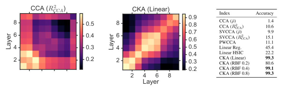
Here is a figure from Kornblith et al. 2019, showing how CKA is much better than CCA for distinguishing neural network layers:
The decoding perspective
The contribution of this paper is to show that we can view these metrics and others from a downstream decoding perspective. Specifically, we can consider decoding a given stimulus input signal from the responses present in a given area. We can call that the area’s representation of that input. One way of understanding the approach in this paper is to compare datasets by correlating their representations of the same input.
A dataset forms a representation of an input through a linear combination of its samples. Some inputs will be easy to construct for a dataset because it has many similar examples available. Others will be more expensive because it will require exploiting unusual directions. These costs therefore reflect the geometry of the dataset and will manifest its representation of the input signal. By comparing these representations, for example by finding the signal that produces the largest agreement, or the smallest, or computing the average agreement, we implicitly compare the geometry of the datasets.
Decoding from a population
Suppose we had $M$ stimuli, each of which contained some known level of a particular feature. We can store these levels in the $M$-dimensional vector $z$.
We can now return to our dataset $X$ of responses to these $M$ stimuli and ask whether a downstream neuron can linearly decode our feature vector $z$ from these activities. We can formalize this as a regression problem, $$\min_w \|z – X w\|_2^2.$$
Now rather than performing the minimization, let’s first reformulate the objective. If we expand it out, we get $$ \|z – X w\|_2^2 = z^T z – 2 z^T X w + w^T X^T X w.$$ The first term doesn’t depend on $w$, so we can drop it and focus on the rest. The second term measures the alignment of $z$ with our proposed readout $Xw$. If we only had this term we could make the objective arbitrarily large or small by scaling $w$.
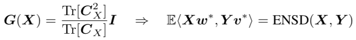
Thankfully, we have the final term, which serves as a cost on $w$. So we can equivalently view our regression problem as a maximization, $$ \max_w 2 z^T X w – w^T G(X) w, $$ where we’ve defined $$G(X) \triangleq X^T X = \Sigma_X.$$
If we add a weight regularizer $\lambda w^T w$ to our original problem, this just gets added in to this penalty metric as $$ G(X) = X^T X + \lambda I.$$ The effect of the penalty can then be seen as $$ w^T G(X) w = w^T X^T X w + \lambda w^T w.$$ Since $Xw$ is our decoded output, we can see this as combining a regularization of the decoder output and the decoder weights. For most of the paper, we’ll be working with penalties of the form $$G(X) = a X^T X + b I.$$
Returning to our optimization problem, the solution is $$ w^* = G(X)^{-1} X^T z,$$ and our estimate of the feature vector is $$ z_X = X w^* = X G(X)^{-1} X^T z = K_X z,$$ where we’ve defined $$ K_X = X G(X)^{-1} X^T.$$
Remark. Notice that for $b = 0$ this is the orthogonal projector onto the column span of $X$. So, if we had as many neurons as stimuli, and our responses weren’t degenerate, we could always recover the input exactly. This highlights the importance of the weight regularization in imposing a scale. In the general case when we have at least as many neurons as stimuli (so $G(X)$ is not necessarily invertible and we need to regularize), we can decompose $X$ as $U_X S_X V_X^T$, in which terms $$ K_X = U_X S_X V_X^T V_X (a S^2_X + b I)^{-1} V_X^T V_X S_X U_X^T = U_X {S^2_X \over a S_X^2 + b I} U_X^T.$$ Directions where $S_X^2 \ll b/a$ will get squished towards zero. This can highlight differences between datasets, even when we have as many neurons as stimuli.
Comparing populations
To compare two sets of population responses, we can simply perform the same decoding analysis on the second set of responses, $Y$, get an optimal set of decoder weights $v^*$, and a corresponding optimal estimate, $z_Y = Y v^*$. We can then compare these estimates with the scalar product, $$ \langle z_x, z_y \rangle = \langle X w^*, Y v^* \rangle = z^T K_X^T K_Y z.$$
In other words, we’ve turned our comparison problem into a decoding problem by asking: How much do decoded outputs agree?
We can answer this question in several ways. We can ask for the best case scenario: what’s the largest agreement we can achieve? We can also ask what the smallest agreement we can achieve is. The answer to both of these questions is easy, once we notice that $$ z^T K_X^T K_Y z = {1 \over 2} z^T(K_X^T K_Y + K_Y^T K_X) z.$$ The matrix in brackets is symmetric, so has real eigenvalues, and the quantities we’re after correspond to the largest and smallest eigenvalues of that matrix. We can then pick out the corresponding eigenvectors as the most agreeable and most disagreeable stimuli. Remark: In fact, we get an eigenbasis of agreeability, going from the most to the least.
We can also ask about the average case. That is, $$ \EE_z z^T K_X^T K_Y z = \EE_z \tr (K_Y zz^T K_X^T).$$ If we assume that $z \sim N(0, I)$, then this expectation is simply the trace of the kernel overlaps, $$ \EE_{z \sim N(0, I)} \tr(K_Y zz^T K_X^T) = \tr(K_Y K_X^T) = {1 \over 2}\tr(K_Y K_X^T + K_X K_Y^T).$$
We can optionally normalize this overlap into a correlation by normalizing it with the norms of the two representations, so \begin{align*}{ \EE_z z^T K_X^T K_Y z \over \sqrt{\EE_z \langle K_X z, K_X z \rangle } \sqrt{\EE_z \langle K_Y z, K_Y z \rangle} } &= {\tr( K_X^T K_Y) \over \sqrt{\tr(K_X^T K_X)} \sqrt{\tr(K_Y^T K_Y)}} \\ &= {\langle K_X, K_Y \rangle \over \|K_X\| \|K_Y\|}.\end{align*}
Similarity measures from decoding
We now see that the expected correlation of decoded vectors is the inner product of the corresponding kernel matrices. We saw earlier that CCA and CKA were themselves such inner products. Therefore, we can view these metrics as average decoding correlations under different penalty regimes.
For example, we saw that CCA compares whitened responses of the form $X \Sigma_X^{-1} X^T.$ This corresponds to $G(X) = \Sigma_X$, or a setting where we penalize only the decoder output, not the synaptic weights.
CKA drops the whitening and compares the raw response correlations $XX^T$. This corresponds to $G(X) \propto I$, where we penalize only the synaptic weights.
Interpolating between the two, so $G(X) = \Sigma_X + \lambda I$, corresponds to the expected euclidean distance between the two decoded representations, equivalently the squared difference between the two decoding kernels, and gives the recently proposed GULP metric.

Expected Number of Shared Dimensions corresponds to a covariance dependent penalty on the readout weights,
Finally, the authors considered the Procrustes distance between two datasets, defined as the minimum distance when allowing for rotations, $$ P(X,Y) = \min_R \|X – Y R\|_F^2,$$ and showed that it was approximately monotonic in the decoding distance.
Conclusion
The authors show how a number of measures for comparing population responses can be viewed from a linear decoding perspective, with each measure corresponding to a correlation of decoded outputs produced using metric-specific costs on those outputs and the synaptic weights used to produce them.
$$\blacksquare$$
Leave a Reply