The low-rank hypothesis of complex systems

In this post I will summarize the paper “The low-rank hypothesis of complex systems” by Thibeault et al.

The authors appear to be coming from the complex-systems / network science. Their argument is as follows:

• Many real world networks have low rank interaction matrices.
• Several important random matrix models are an element-wise function of a low rank matrix, plus noise, and remain low-rank.
• Low rank interactions suggests low-dimensional dynamics.
• These are found by aligning a to-be-determined low-dimensional vector field with some aspect of the high-dimensional one.
• The most natural way to do this is complicated.
• Solving a related problem they arrive at $F^*(X) = M f(M^\dagger,X)$ for projection matrix $M$.
• Use this to show how the error is bounded by the singular values.
• When the projection is aligned with the connectivity matrix $W$, the low-dimensional projection can exactly capture the high-dimensional one in some important cases, including RNNs.
• Their ansatz also implies higher-order interactions of the low-dimensional observables.

Many real world networks have low effective rank

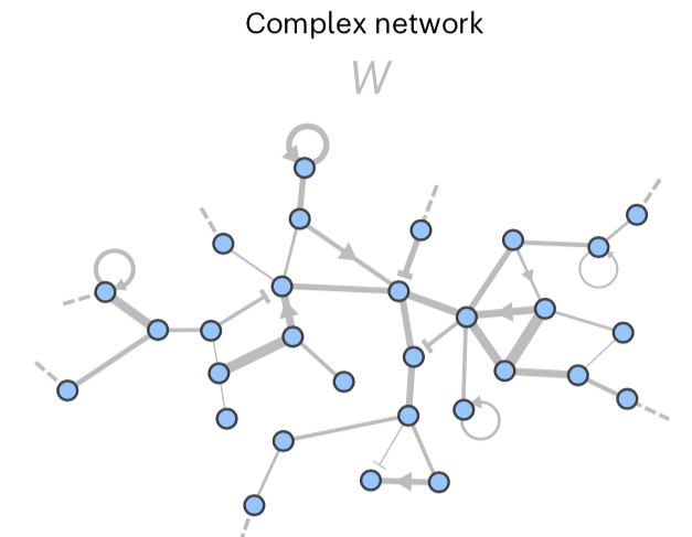
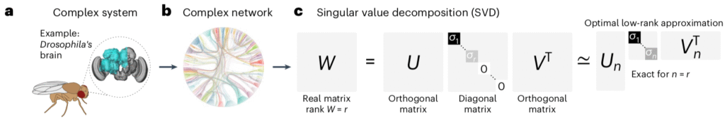
Many complex systems consist of a large number of interacting units. The interactions of these units can often be described by a matrix W indicating the influence of each unit on every other. This is schematized below.

The interactions defined by W can be complex. This complexity can be measured by the singular values of W, specifically by how quickly they decay. The singular values determine the best-low rank approximation of W.

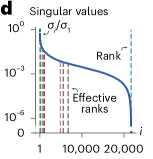
Therefore, the faster the singular values decay the more structured it is. The rapidity of decay can be quantified into various measures of effective rank. For example, the stable rank measures the cumulative sum of squares of the singular values normalized by the largest. The decay of the singular values, along with various measures of effective rank, computed for the connectome above, are shown below.

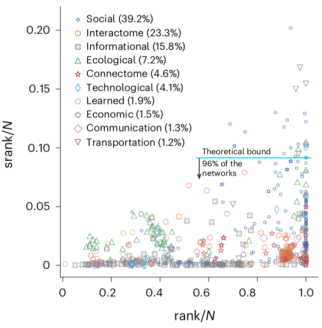
It turns out that many real-world networks have low effective rank. The authors examined ~700 such networks and computed the statistics of singular value decay, shown below:

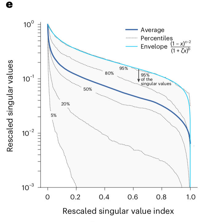
The stable rank of these is typically 10% or less of the ambient rank.

Many random graphs are built atop low-rank matrices

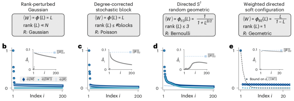
Many random graph models can be decomposed as an element wise function of a low rank matrix, corrupted by additive noise.

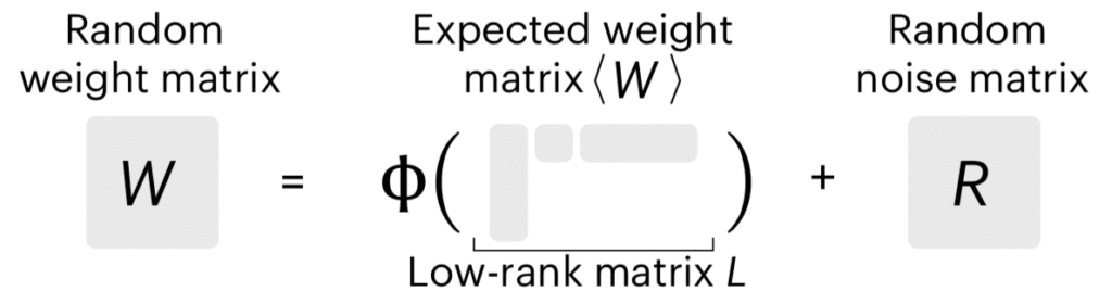
Despite the element-wise function and the additive noise, the resulting weight matrices retain their low-ranked-ness, partially due to Weyl’s theorem showing that singular values are robust to additive perturbations.

The low-dimension hypothesis

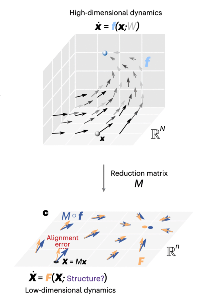
Low rank structure in the interactions among units suggests that the dynamics of such a system may have low dimensional structure. Specifically, we hope to find a low-dimensional linear projection of the activity, defined by the $n \times N$ matrix $M$, that matches the high-dimensional dynamics. That is, given dynamics $$\dot x = f(x),$$ we hope to find $X \triangleq M x$ whose dynamics $$\dot X = F(X)$$ match the original in some least squares sense.

One natural way to do this is to project the complete dynamics and compare them to the reduced dynamics, $$ \mathcal{E}(x) = \|M f(x) – F(M x)\|.$$ This is shown schematically below.

A dimension reduction ansatz

However, minimizing this over $M$ and $F$ is hard. Instead, we consider lifting the low-dimensional dynamics to the complete space using the pseudo-inverse $M^\dagger$ of the projection and comparing it to the complete dynamics on the projection, so $$ \veps(x) = \|f(Px) – M^\dagger F(M x)\|,$$ where $P = M^\dagger M$ is the projection from $\RR^n \to \RR^N$. It turns out that this has a simple solution. Since $$f(Px) = f(M^\dagger M x) = f(M^\dagger X),$$ we can write the above error as $$ \veps(x) = \|f(M^\dagger X) – M^\dagger F(X)\|.$$ So we just set $$ F^*(X) = M f (M^\dagger X).$$

Bounding the reconstruction error

We can now bound the error we’re interested in for this particular choice of vector field. Before doing so, we make one more assumption to make the dependence on the structure expliction, that the dynamics are of the form $$ f(x) = g(x, y), \quad y = W x.$$ Defining the projections $$\hat x \triangleq M x, \quad \text{and} \quad \hat y \triangleq M y,$$ our error is $$ \mathcal{E}(x) = \|M g(x,y) – M g(\tilde x, \tilde y)\| = \| M [g(x,y) – g(\tilde x, \tilde y)] \|.$$

The difference in the vector fields can be described using the jacobians of g as $$ g(x,y) – g(\tilde x, \tilde y) = J_x (x – \tilde x) + J_y (y – \tilde y) = J_x (x – \tilde x) + J_ y W (x – \tilde x),$$ where the Jacobians are evaluated at some intermediate point between $\tilde x$ and $x,$ and $\tilde y$ and $y.$ Also, $$x – \tilde x = x_\perp = (I – P) x, \quad P = M^\dagger M.$$ So our error becomes $$ \mathcal{E}(x) = \|M g(x,y) – M g(\tilde x, \tilde y)\| = \| M J_x (I – P) x + M J_y W (I – P) x \|.$$

We can use the triangle inequality to split this up into two components,$$ \mathcal{E}(x) \le \| M J_x x_\perp\| + \|M J_y W x_\perp \|.$$

To bring $W$ further into the picture, we split the second component further, so $$ \mathcal{E}(x) \le \| M J_x x_\perp\| + \|M J_y\| \| W x_\perp \|.$$

Now if we set $M = V_n^T$, the first $n$ singular vectors of $W$, then we can bound the last term, so $$ \mathcal{E}(x) \le \| M J_x x_\perp\| + \sigma_{n+1} \|M J_y\| \|x_\perp\|.$$

Exact reconstruction

From this, we get that if $J_x \propto I$, the first term is zero, and $n = \text{rank}(W)$ makes the second term zero. So our ansatz vector field gives exact reconstruction in those cases. An important example of this is for RNNs, with dynamics like $$ \dot x = -x + s(W x),$$ for $W = U S V^T$ of rank $n$ and some fixed function $s$ that can include inputs to each unit. Our ansatz says that this can by exactly dimension reduced using $$ \dot X = -X + V^T s( U \Sigma X), \quad X = V^T x.$$ An example of this is shown below. The black data is the bound, the blue data are the singular values of $W$, and the reconstruction error is in red.

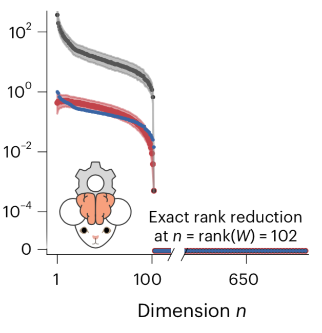
This shows that at least in some important special cases, low rank $W$ produces low-dimension dynamics.

The general case

More generally, using $\|x_\perp\| \le \|x\|$ and $\|M\| \le 1$, we get $$ {\mathcal{E}(x) \over \|x\|} \le \| J_x \| + \sigma_{n+1} \|J_y\|.$$ We can reduce this bound by using a projection that has the same rank as our interactions matrix. This eliminates the second term, but the first term remains, and we’re no longer guaranteed to reduce reconstruction error to zero. Examples of this more general case are shown below:

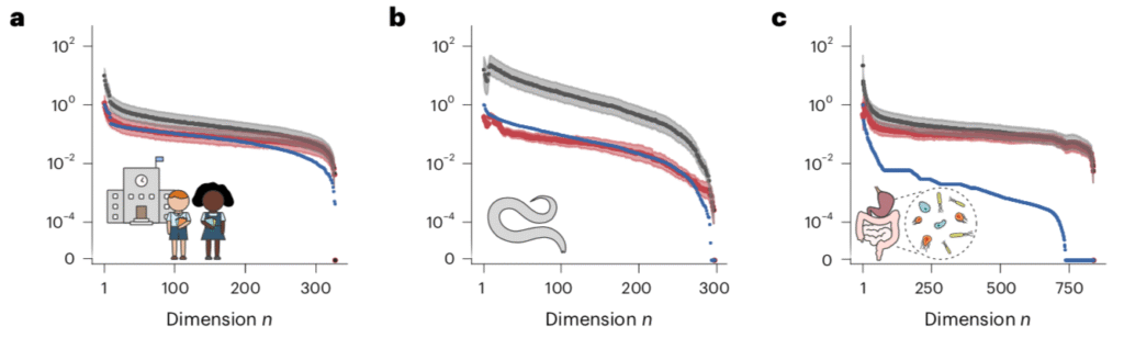
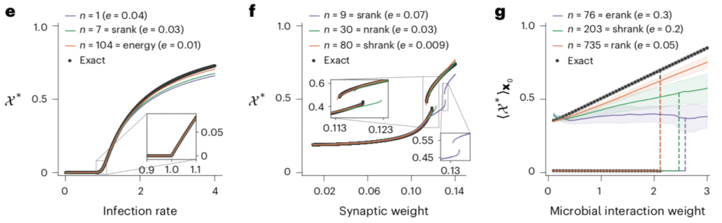
Despite the non-zero reconstruction error, the ansatz is still able to capture important dynamical properties, such as bifurcations, in each system:

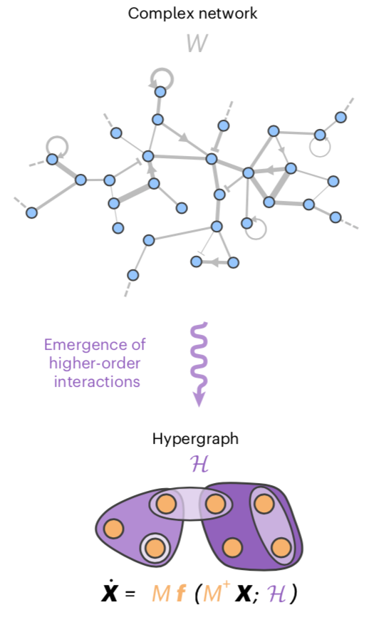
Dimension reduction leads to emergence of higher-order interactions

The final point the authors make is that dimension reduction of dynamics on a network can produce higher-order interactions. This is shown schematically below:

To see how this comes about, we start with our high dimensional network dynamics. The activity of each of the $N$ nodes is a function of its own activity, and a weighted combination of the rest of the nodes, $$ \dot x_i = h_i(x_i, y_i), \quad y_i = \sum W_{ij} x_j.$$ If we assume that the $h_i$ are analytic functions, we can write it as

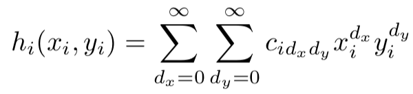
Under our ansatz $\dot X = M f(M^\dagger X),$ the reduced dynamics then become,

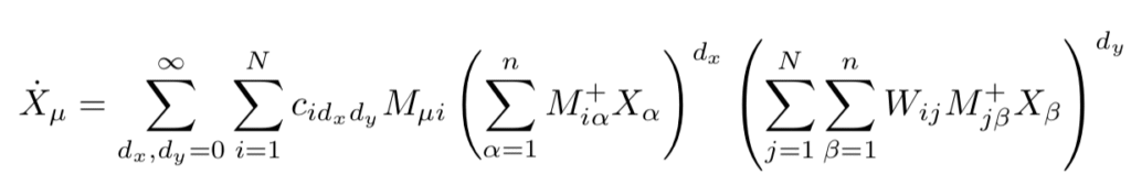
and expanding the terms in brackets yields the higher-order interactions.

Summary

In summary, the authors

1. Provide empirical evidence that many real world networks, and some models of random matrices, have low effective rank.
2. By using an ansatz for dimension-reduction of the high-dimensional vector field, show that low-effective rank of connectivity can, in some important cases, imply low-dimensional dynamics, capturable by projection onto a subspace determined by the connectivity.
3. Show that such dimension reduction can generically produce high-order interactions among the observables.