We’re trying to understand the solutions when minimizing $$L(\zz) = {1 \over 2 M^2} \|\XX^T \ZZ^2 \XX – \SS\|_F^2 + {\lambda \over 2 N}\|\zz – \bone\|_2^2.$$
We can write this as $$L(\zz) = {1 \over 2 M^2} \|\RR \zz^2 – \ss \|_2^2 + {\lambda \over 2 N}\|\zz – \bone\|_2^2,$$ where the $i$’th column of $\RR$ is the vectorized representational atom contributed by unit $i$, $\vec{\XX_i \otimes \XX_i}$, and $\ss = \vec{\SS}$.
When we run the minimization, we get results like this:
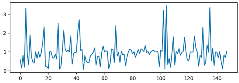
We’d like to understand why some units are boosted, while others are set to zero.
To do so we’d normally set the derivative to zero and interpret the result, but the result is a cubic equation which is hard to interpret. So instead, in this post we’re going to apply a quantization approach: map $z_i$ to a few discrete values and see if we can understand why those values were chosen.
Quantization
We’re going to assume that $z_i \in [0, 1, z]$, for some as yet to be determined $z > 1$. These values were chosen because 0 means a channel is being suppressed, 1 means regularization is contributing nothing, and $z$ indicates the large values. We will consider the conditions that the $i$’th channel must satisfy to have those values.
Let $\hat \ss = \RR \zz^2$, and $\hat \ss_{i} = \RR_{/i} \zz_{/i}^2$, and $\rho_i = {\lambda \over 2 N}\|\zz_{/i}-\bone\|_2^2$. Multiplying everything by $2M^2$ and relabeling $\lambda \to \lambda M^2 / N$, we get \begin{align}L(z_i=k) &= \|\ss – \hat \ss_i – \RR_i k^2\|_2^2 + \rho_i + \lambda (k – 1)^2\\&= \Delta_i^2 -2 \Delta_i^T \RR_i k^2 + \RR_i^2 k^4 + \rho_i + \lambda (k-1)^2.\end{align}
Removing the common factor of $\Delta_i^2 + \rho_i$, we have \begin{align}L_i(0) &= \lambda,\\ L_i(1) &= – 2\Delta_i^T \RR_i + \RR_i^2, \\ L_i(k) &= – 2 \Delta_i^T \RR_i k^2 + \RR_i^2 k^4+ \lambda (k-1)^2.\end{align}
Let’s first consider when $z_i=0$ wins out. This is when $L_i(0) < L_i(1)$ and $L_i(0) < L_i(k).$
\begin{align} L_i(0) < L_i(k) \implies \lambda &< – 2\Delta_i^T \RR_i k^2+ \RR_i^2 k^4 + \lambda (k-1)^2\\\implies \Delta_i^T \RR_i &< {\RR_i^2 k^4 + \lambda((k-1)^2 – 1)\over 2 k^2 }\\ &= {\RR_i^2 k^3 + \lambda(k – 2) \over 2 k }\\
&= {1 \over 2} \RR_i^2 k^2 + {\lambda_k \over 2}\\ &\triangleq \theta_i(k).\end{align} where I’ve defined $$\lambda_k = \lambda {k – 2 \over k}.$$
To make our life easier let’s assume that $k$ is such that $\theta_i(k) > \theta_i(1)$. We must have \begin{align}\RR_i^2 k^2 + \lambda_k &> \RR_i^2 – \lambda.\\
\RR_i^2 (k^2 – 1) &> -\lambda {k -2 + k \over k} = -\lambda {2 (k -1) \over k} \\\RR_i^2 (k + 1) &> -\lambda {2 \over k}.\end{align}
But the LHS is positive and the RHS is negative, so this will always hold. So to determine whether to drop an element, I only need to compare it to $L_i(1)$. If it’s less than that, then it will automatically be less than $L_i(k)$, so I should drop it. If it’s not less than that, then I should include it, either at the unit or $k$ level.
We can consider building up the estimate $\hat s$ one at a time.
I can imagine going through the indices in sequence. The current estimate, before I make the $i$’th decision, is $\hat \ss_i$. The current error, is $\Delta_i$.
Since including an element at unit concentration doesn’t incur a regularization penalty, that will be the default choice.
If I choose to drop the element, I must have that $L_i(0) < L_i(1)$, or $$ \Delta_i^T \RR_i < {\RR_i^2 -\lambda \over 2},$$ or in terms of unit vectors, $$ \Delta_i^T \hat \RR_i < {\|\RR_i\| \over 2} – {\lambda \over 2 \|\RR_i\|}.$$
When the $\RR_i$ is large, the threshold will tend to half the norm. So a large $\RR_i$ will be dropped unless the overlap is at least half its size.
When $\RR_i$ is small, the RHS will tend to $-\lambda/2\|\RR_i\|$. So $\RR_i$ will tend to be kept. To be dropped, its unit vector must at least be in the opposite opposite direction to the residual.
Small and large are determined by $$\|\RR_i\| \gg \lambda / \|\RR_i\| \iff \|\RR_i\|^2 \gg \lambda.$$
When we look at the results, that is indeed the broad trend that we see:
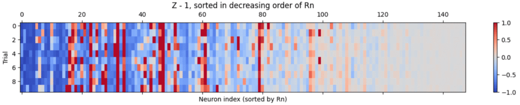
Units with larger norms, on the left, tend to be suppressed, while those with smaller norms, on the right, tend to be kept.
Now suppose a unit hasn’t been dropped. Then it’s either let through unchanged, or amplified by $k$. To let it through as is, we must have $ L_i(1) < L_i(k),$ or \begin{align} – 2\Delta_i^T \RR_i + \RR_i^2 &< – 2 \Delta_i^T \RR_i k^2 + \RR_i^2 k^4+ \lambda (k-1)^2\\ 2 \Delta_i^T \RR_i (k^2 – 1) &< \RR_i^2 (k^4 – 1) + \lambda (k-1)^2 \\ 2 \Delta_i^T \RR_i &< \RR_i^2 (k^2 + 1) + \lambda {k-1 \over k + 1}\\ \Delta_i^T \hat \RR_i &< {\|\RR_i\| (k^2 + 1) \over 2} + {\lambda \over 2 \|\RR_i\|} {k-1 \over k + 1}\end{align}
Again we do a small/large analysis. Large here will mean \begin{align}\|\RR_i\| (k^2 + 1) &\gg {\lambda \over \|\RR_i\|} {k-1 \over k + 1}\\
\|\RR_i\|^2 &\gg \lambda {k – 1 \over (k^2 + 1) (k+1)}
\end{align}
If the unit is large, then the overlap with the residual must be $(k^2 + 1)/2$ times its size, otherwise it will be left unamplified.
If the unit is small, then its overlap with the residual must be larger than than the right hand term, otherwise it will stay at 1.
In particular, the largest the lefthand side can be is $\|\Delta_i\|$, which, if we assume residuals are getting smaller after each step, will be at most $\|\ss\|$. So any units for which $$ \|\RR_i\| \le {\la \over 2 \|\ss\|}{k – 1 \over k + 1}$$ will never be amplfied. We’ll call these tiny.
That distinction doesn’t seem to pan out in the data – the tinyness threshold is quite high (red in the plot below):
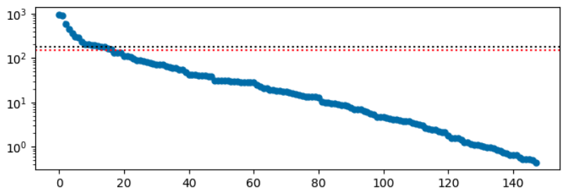
But clearly many units with norms below this threshold are amplified. So something is off with that analysis…
Either way, raw overlap is not a good measure of whether a unit was amplified or not:
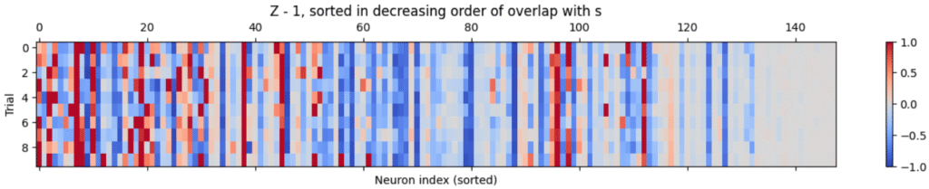
But that’s to be expected.
One advantage of our approach is that it reduces our estimate to two vectors, $$\hat \ss = \rr_1 + \rr_k, \quad \rr_1 \triangleq \sum_{i \in I_1} \RR_i, \quad \rr_k \triangleq \sum_{i \in I_k} \RR_i, \quad \rr_0 \triangleq \sum_{i \in I_0}\RR_i.$$
We can then ask, e.g. what the lengths of each of these components is, and what its overlap with the target, $\ss$, is. We would expect, for example that $\rr_0$ doesn’t overlap strongly with $\ss$.
To try to get at some of that information, we can appeal to stability conditions, that say that, given our solution set, promoting or demoting any unit would be costly.
Let’s start with the units that are suppressed. We have, by definition, that promoting any of them would cost more than leaving them out. So we have, in the notation above, that $$L_i(1) – L_i(0) > 0 \quad \forall i \in I_0.$$ Using our expressions for these above, we therefore find that $$ 2 \Delta_i^T \RR_i <\RR_i^2 – \lambda \quad \forall i \in I_0.$$ For this group, $\Delta_i$ is $\Delta = \ss – \rr_1 – \rr_k$, since after our choice (to keep these units inactive), the active set doesn’t change.
In particular, we get $$ 2 (\ss – \rr_1 – \rr_k)^T \RR_i < \RR_i^2 – \la \quad \forall i \in I_0.$$
This is one inquality per unit, so we might come back to it later to extract the details. For now, we’ll sum over all units to get one inequality about $\rr_0$: $$ 2(\ss – \rr_1 – \rr_k)^T \rr_0 < \sum_i \RR_i^2 – n_0 \la.$$ Rearranging, we get $$\boxed{ 2 \ss^T \rr_0 < 2 \rr_0^T(\rr_1 + \rr_k) + \sum_{I_0} \RR_i^2 – n_0 \la.}$$
Next, we consider the units in $I_1$. These don’t get promoted or demoted. For these units, $\Delta_i$ is missing their contribution to $\Delta$: $$\Delta = \Delta_i – \RR_i \implies \Delta_i = \Delta + \RR_i.$$
First, we have that they don’t get demoted. So $$L_i(0) – L_i(1) > 0 \quad \forall i \in I_1.$$ Recalling that $L_i(k) = -2 \Delta_i^T \RR_i k^2 + \RR_i^2 k^4 + \lambda (k-1)^2,$ we have $$ -2 \Delta_i^T \RR_i + \RR_i^2 < \lambda \quad \forall i \in I_1.$$
Plugging in the expression for $\Delta_i$, we get \begin{align} 2 (\Delta + \RR_i)^T \RR_i &> \RR_i^2 – \lambda \\ 2 \Delta^T \RR_i &> -\RR_i^2 – \lambda \\ 2(\ss – \rr_1 – \rr_k)^T \RR_i &> -\RR_i^2 – \lambda\\ 2 \ss^T \RR_i &> 2(\rr_1 + \rr_k)^T \RR_i – \RR_i^2 -\lambda,\end{align} so finally, $$\boxed{2\ss^T\rr_1 > 2(\rr_1 + \rr_k)^T \rr_1 – \sum_{i \in I_1} \RR_i^2 – n_1 \lambda.}$$
Next, we have that they don’t get promoted, so $$ L_i(k) – L_i(1) > 0 \quad \forall i \in I_1.$$ This means \begin{align} -2\Delta_i^T \RR_i + \RR_i^2 &< -2 \Delta_i^T \RR_i k^2 + \RR_i^2 k^4 + \lambda (k-1)^2\\2\Delta_i^T \RR_i (k^2 – 1) &< \RR_i^2 (k^4 -1) + \lambda (k-1)^2\\2(\Delta + \RR_i)^T \RR_i (k^2 – 1) &< \RR_i^2 (k^4 -1) + \lambda (k-1)^2\\2\Delta^T \RR_i (k^2 – 1) &< – 2 \RR_i^T \RR_i (k^2 – 1)+ \RR_i^2 (k^4 -1) + \lambda (k-1)^2\\&= \RR_i^2 (k^4 -2k^2 +1) + \lambda (k-1)^2\\&= \RR_i^2 (k^2 – 1)^2 + \lambda (k-1)^2\\2\Delta^T \RR_i &< \RR_i^2 (k^2 -1) + \lambda {k-1 \over k+1}\\2(\ss – \rr_1 – \rr_k)^T \RR_i &< \RR_i^2 (k^2-1) + \lambda {k-1 \over k+1}\\2 \ss^T \RR_i &< (\rr_1 + \rr_k)^T \RR_i +\RR_i^2 (k^2-1) + \lambda {k-1 \over k+1},\end{align} so we finally arrive at $$\boxed{2 \ss^T \rr_1 < 2 (\rr_1 + \rr_k)^T \rr_1 +\sum_{i \in I_1}\RR_i^2 (k^2-1) + n_1 \lambda {k-1 \over k+1}.}$$
Finally, we have that the units in $I_k$ don’t get demoted. That is $$ L_i(1) – L_i(k) > 0 \quad \forall i \in I_K.$$ For these units, $\Delta = \Delta_i + k^2 \RR_i.$ So we then have \begin{align} -2\Delta_i^T \RR_i + \RR_i^2 &> -2 \Delta_i^T \RR_i k^2 + \RR_i^2 k^4 + \lambda (k-1)^2\\2\Delta_i^T \RR_i (k^2 – 1) & > \RR_i^2 (k^4 -1) + \lambda (k-1)^2\\2(\Delta + k^2 \RR_i)^T \RR_i (k^2 – 1) &> \RR_i^2 (k^4 -1) + \lambda (k-1)^2\\2\Delta^T \RR_i (k^2 – 1) &> -2 k^2 \RR_i^T \RR_i (k^2 – 1)+ \RR_i^2 (k^4 -1) + \lambda (k-1)^2\\&= \RR_i^2 (-k^4 +2k^2 -1) + \lambda (k-1)^2\\&= -\RR_i^2 (k^2-1)^2 + \lambda (k-1)^2\\2\Delta^T \RR_i &> -\RR_i^2 (k^2 -1) + \lambda {k-1 \over k+1}\\2(\ss – \rr_1 – \rr_k)^T \RR_i &> -\RR_i^2 (k^2 – 1) + \lambda {k-1 \over k+1}\\2 \ss^T \RR_i &> (\rr_1 + \rr_k)^T \RR_i -\RR_i^2 (k^2 -1) + \lambda {k-1 \over k+1},\end{align} and we finally arive at $$\boxed{2 \ss^T \rr_k > 2 (\rr_1 + \rr_k)^T \rr_k -\sum_{i \in I_k}\RR_i^2 (k^2-1) + n_k\lambda {k-1 \over k+1}.}$$
All of these expressions have told me about the projections of $\Delta$ onto $\rr_1$ and $\rr_k$ – but I’d like to know about the projections of $\ss$ onto these individually…
If we plot the solution coefficients against the norms of the represenations, we get something like this:

We’ve got an expanation of the general trend, which shows the weak representations going through unchanged, while the strong ones tend to get suppressed. What about the ones in the middle, that are amplified?
Returning to $L_i(k)$, we can compute the derivative and get \begin{align} {d L_i \over dk} &= -4 \Delta_i^T \RR_i k + 4 \RR_i^2 k^3 + 2 \lambda (k-1)\\ &= 4 \RR_i^2 k^3 + (2\lambda -4 \Delta_i^T \RR_i) k -2 \lambda \end{align}
Setting this to zero, we get $$ k^3 + {{1 \over 2}\lambda- \Delta_i^T \RR_i \over \RR_i^2}k – {\lambda \over 2 \RR_i^2} = 0, \quad \checkmark$$ which we can also write as $$ k^3 – {\Delta_i^T \RR_i \over \RR_i^2} k + {\lambda (k – 1) \over 2\RR_i^2}.$$
It will be useful below to write $$ \Delta_i ^T \RR_i = (\ss – \ss_i)^T \RR_i = (\ss – \ss_i)^T \hat \RR_i \|\RR_i\| = (a_i – \hat a_i) \|\RR_i\|,$$ where $a_i$ is the alignment of the $i$’th unit with the target, while $\hat a_i$ is its alignment with the estimate (that doesn’t include it).
We can now split this into three regimes.
If $k$ is very small, then $k^3 \approx 0$, and we can approximate the equation as $$ -\Delta_i^T \RR_i k = {\lambda \over 2},$$ or in terms of alignments
$$ (\hat a_i – a_i) \|\RR_i\|k = {\lambda \over 2} \implies k = {\lambda \over 2 \|\RR_i\|(\hat a_i – a_i)}.$$
If $k$ is large, then we can approximate the solution by dropping the last term. In that case, we get
$$ k^2 = {2 \Delta_i^T \RR_i – \lambda \over 2 \RR_i^2} = {\hat \RR_i^T (\ss – \hat \ss_i) \over \|\RR_i\|} – {\lambda/2 \over \RR_i^2} = {a_i – \hat \RR_i^T \hat \ss_i – {\lambda \over 2 \|\RR_i\|} \over \|\RR_i\|}.$$
$$\blacksquare$$
Leave a Reply