These notes are about analyzing the fluctuations of patch current to determine the number and unitary current of the underlying ion channels. They are based on these notebooks, which in turn are based on this tutorial on fluctuation analysis. The techniques involved are simple and generalize to other contexts.
Our context is a patch-clamp experiment in voltage-clamp, in which we apply a voltage to the patch and measure the current across it.
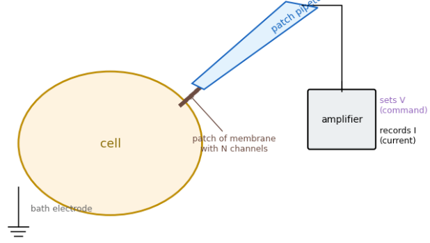
Current can flow due to the presence of ion channels spanning the membrane. Some channels are open all the time. Others transition between conductive (open) and non-conductive (closed) states. Those are the ones we’ll be interested in here. In particular, we’re interested in the current a channel conducts in its open state, the so-called unitary current.
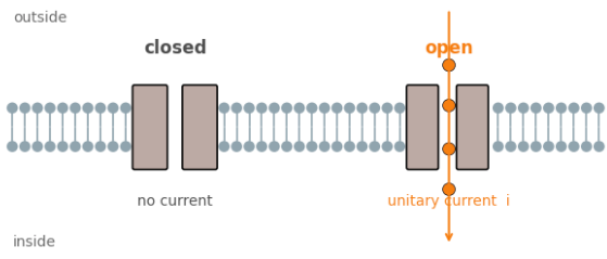
In the simplest case, which we’ll consider here, there is just a single open state, and a single closed state.
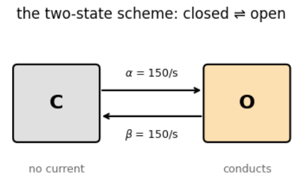
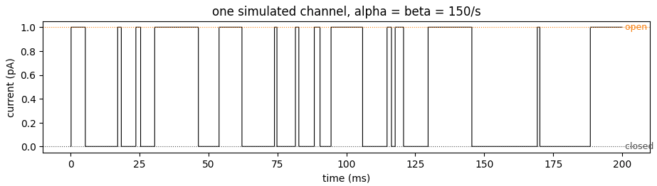
The channel flips back and forth between the two states in a memory-less way, according to their given rates. Both are $150/s$ in the example above, though they don’t have to be equal in general. This produces a flickering current signal,
As the transition rate $\alpha$ from closed to open increases relative to the rate from open to closed, the channel remains open more and more.
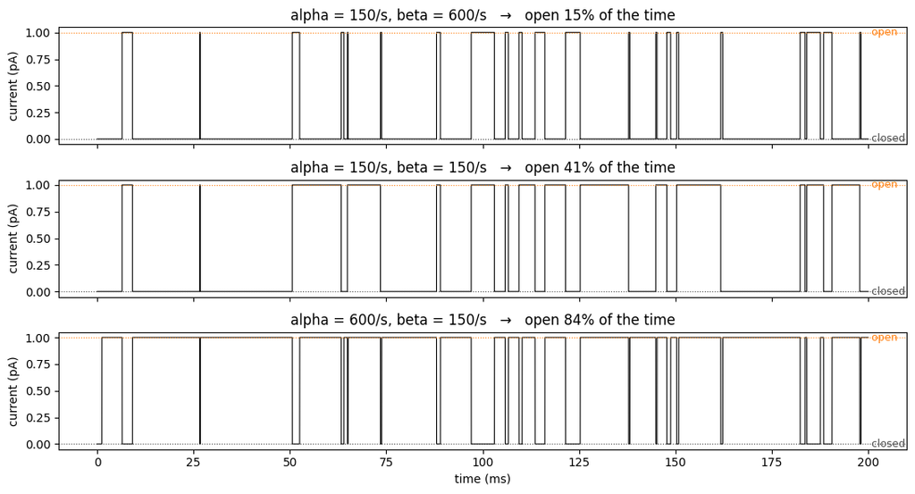
The open probability is $$ p = {\alpha \over \alpha + \beta}.$$ The average current through the channel is then the full unitary current, scaled by the open probability, $$ \langle I\rangle = p i.$$
For voltage-dependent channels, the open probability is voltage specific. For the ones we consider here, the higher the voltage, the higher the open probability:
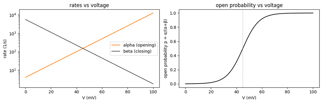
Recall that we’re after the unitary current, $i$. It seems easy to read this off from the measurements above: increase the voltage high enough so all channels are open, then read off the average current: $\langle I \rangle = i p = i 1. = i.$
More channels, more problems
The problem is that a real patch isn’t going to have just a single channel, but many, say $N$. The mean current is then $N i p$, or $N i$ when all channels are open.
We want to estimate $i$, but is tied up with $N$. That is, is the current coming from one large channel, with current $N i$, or $N$ small single channels, or something else?
The solution to this problem is to use not just the mean of the current, but the variance of the current as well.
The intuition is that if it was one large channel, it would be flickering between on and off, lots of variance. If $N$ single channels, individual flickerings would tend to cancel out, giving a smoother current.
Measuring the variance, $\sigma^2$, of the current in each situation makes this explicit. In particular, we have,
- The variance of one channel with unitary current $i$: $\; i^2 p(1 – p)$.
- The variance of $N$ channels with unitary current $i$: $\; N i^2 p (1 – p).$
- The variance of one channel with unitary current $Ni$: $\; N^2 i^2 p(1 – p).$
Notice that the last two cases have the same mean current. But the variance produced by the single, large, channel is much greater ($N$-times) than that of the $N$ small channels.
We now have an equation for the mean, and one for the variance:
- $\langle I \rangle = N i p$.
- $\sigma^2 = N i^2 p(1 – p)$.
We could compute these quantities by e.g. using the voltage-clamp to set the membrane at some intermediate voltage, waiting for the open probabilties to equilibrate to their new value, and the measuring the mean and variance of the current over some fixed time interval.
That would give us two equations, for three unknowns ($N$, $i$, $p$). We could repeat the procedure at another voltage. This would yield two more equations, but only one more unknown, $p$ at the new voltage. We would thus have four equations in four unknowns, and could solve for the unknown variables, including $i$ and $N$.
Sweeps to the rescue
While this procedure would work in theory, it requires (a) choosing two voltages (why two, why not more?), (b) waiting for the system to equilibrate, and (c) picking some time interval to compute means and variances over.
A more elegant procedure that avoids all of these problems uses the fact that when a voltage step is applied, it takes some time for the channels to arrive at their new open probabilities.
From the rate equation for the channels, we can read off that $$ {d p \over dt} = (1 – p) \alpha – \beta p.$$ We can express this slightly more usefully as $$ {1 \over \alpha + \beta} {d p \over dt} = -p + {\alpha \over \alpha + \beta}.$$
So we can see that when the voltage changes, setting new $\alpha$ and $\beta$ rates, the open probability converges to the new equilibrium probability of $\alpha / (\alpha + \beta)$ with a time constant of $$ \tau = {1 \over \alpha + \beta}.$$
We can see this in action by repeatedly applying a voltage step to a single channel. At any point along each such “sweep”, the channel state is binary, either open or closed. By averaging the state over sweeps, we arrive at the open probability, and can observe it settling exponentially to its new value:
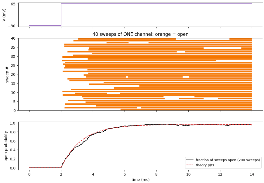
We can apply this same approach to a patch containing $N$ channels. When we repeatedly apply the same voltage step to the patch, the open probability will change exponentially towards its new value. Crucially, it will do so with the same time course each time. An example of this is shown below:
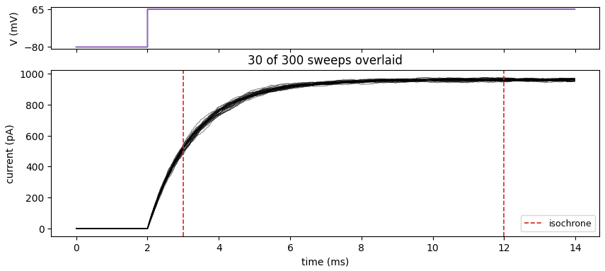
The dashed vertical lines are isochrones, meaning “same time”, in this case measured relative to the voltage onset. The statistics of the current at an isochrone will correspond to the same open probability. Below are the distributions of currents measured in the 300 sweeps for the two isochrones above:
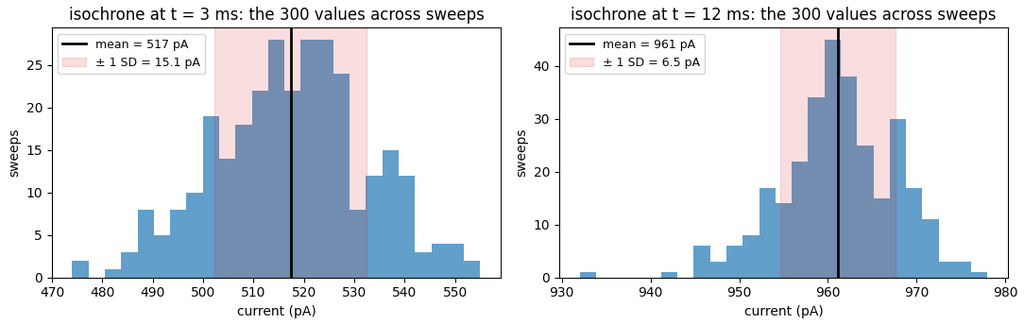
As before, measuring the mean and variance of the current at these two isochrones gives us $2 \times 2 = 4$ equations, for 4 unknowns: $N, i, p_1, p_2$, where $p_1$ and $p_2$ are the open probabilities at the two isochrones.
But why use just two isochrones, when we can use all of them?
To do so, we express the open probability in terms of the mean current. $$ \langle I \rangle = N i p \implies p = {\langle I \rangle \over N i}.$$
This then gives us a relationship between the mean and variance of the current that involves only the unitary current and the number of channels as free variables.
$$ \sigma^2 = N i^2 p(1-p) = i \langle I \rangle – {1 \over N} \langle I \rangle^2.$$
Therefore, variance is a quadratic function of the mean current.
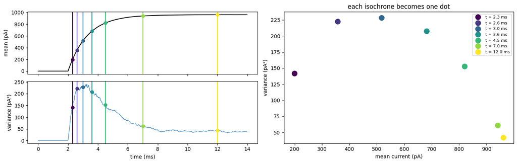
Below we’ve plotted the variance of the current against the mean at a few isochrones:
Plotting the points for all isochrones gives the parabolic relationship:
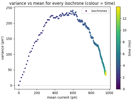
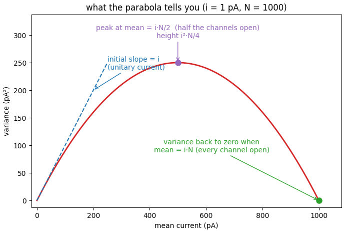
We can read the key parameters straight from the plot. For example, when the mean current is very small, we can ignore the $\langle I \rangle^2$ term, and variance becomes a linear function of the mean current, $$ \sigma^2 \approx i \langle I \rangle, \quad \text{($\langle I \rangle$ very small)}.$$
This small current condition occurs at the left leg of the parabola. The linear relationship tells us that the slope of the parabola at that point is the unitary current.
If we’re interested in the number of channels, we can read that off the plot as well. The variance is zero at both the left and right legs of the parabola. The corresponding values of the mean current satisfy $$ 0 = \sigma^2 = i \langle I \rangle – {1 \over N} \langle I \rangle^2.$$
Solving for the mean current gives $$ \langle I \rangle = 0 \quad \text{or} \quad N i.$$
Therefore, the non-zero value of the current at which the variance is zero is $N i$. This makes sense – it corresponds to the voltage at which the open probability of each channel is 1, and all channels are open.
Having determined the unitary current from the slope at the left leg of the parabola, we can divide the mean current at the right leg by this current to determine the number of channels, $N$.
But we don’t have to use these values to determine $i$ and $N$. We fit the whole curve using linear regression, with the mean current and its square as the predictors and the variance as the target. The coefficients of the mean current and the square will then be $i$ and $-N^{-1}$, respectively.
Real recordings
All of this works in theory. In practice, several problems can come up that will bias the estimates of the patch parameters.
Noisy baseline
The analysis above assumes that there is no noise when the voltage is at the baseline:
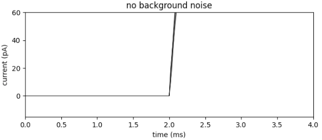
Real recordings can be noisy:
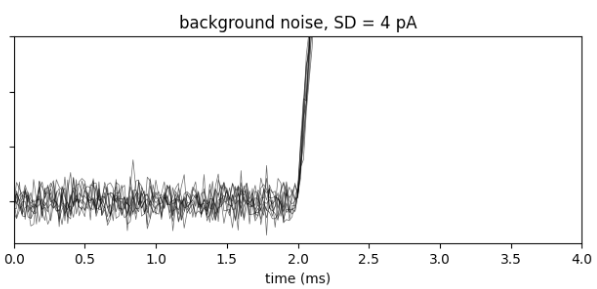
Such additive noise will shift the parabola upwards by the noise variance, so that even at 0 current there will be a non-zero variance. Not accounting for this will bias the estimates:
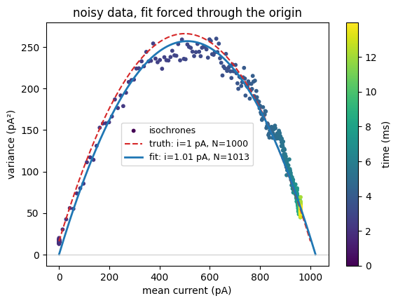
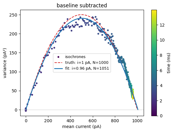
The fix is simple – subtract the baseline variance from the variances at each isochrone before performing the fit.
Rundown
A more interesting problem is rundown. This occurs when the number of channels in the patch decreases over the course of the sweeps. In the example below, we show the current measured at one isochrone over the course of the 300 sweeps:
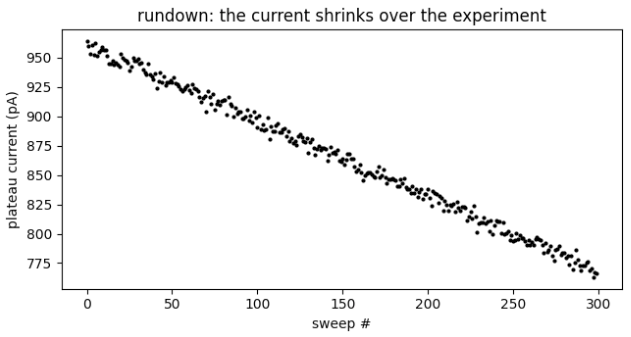
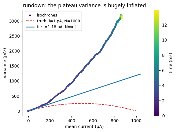
If we measured the variance of this current, it would include, in fact be dominated by, the effect of the rundown, the drop in current from 950 pA to 775 pA.
This effect would be larger at later isochrones than earlier ones, since a larger initial current results in a larger decrease when channels drop out. Plotting the variance against the mean current still produces a parabola, but facing the wrong direction!
We can deal with this by measuring variance in a different way. Rather than measuring the variance of the current measurements themselves, we can measure the variance of the difference in consecutive current measurements.
The intuition is that the rundown between two sweeps should be negligible. And the variance of the difference will then be approximately twice that channel variance we’re after.
To see how this would work for our example above, let’s call the current measured on the $k$’th sweep $x_k$. We can see from the points plotted above that $x_k$ consists of a decreasing linear term, plus some noise scatter: $$x_k = a – b k + \xi_k,$$ where $\xi_k$ is the additive noise with variance $\sigma^2$. This variance is what we’re after.
If we computed the variance of the $x_k$, the result would include the effect of the rundown, the $-bk$ term. Instead, we first compute the difference between successive sweeps:
$$ y_k = x_{k+1} – x_{k} = (a – b(k+1) + \xi_{k+1}) – (a – b k + \xi_k) = -b + \xi_{k+1} – \xi_k.$$
The $-b$ term is constant and doesn’t contribute variance. The two noise terms are independent, so their variances add. Therefore, we can get the variance we’re after by halving the variance of the differences.
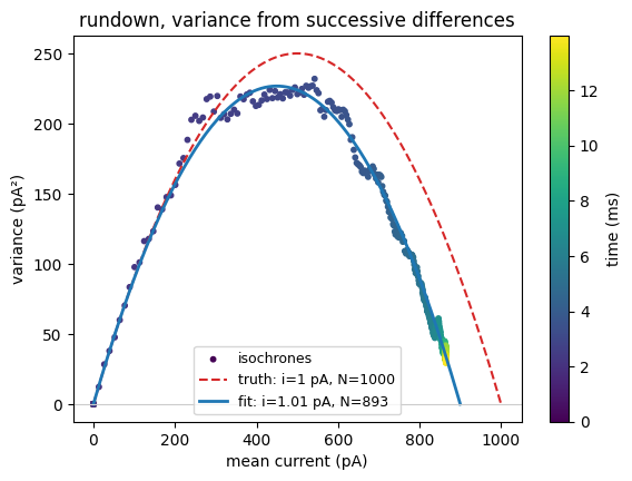
Notice that the estimated number of channels comes out to be the average of the values in the sweep: we started with 1000, ended with 800, and our estimate comes out at about 900.
Stationary Analysis
At this point we’re done – we’ve determined the channel parameters, $i$ and $N$, that we were after.
However, we can go a bit further. Recall that the open probability a channel settled to at a given voltage was $$ p(V) = {\alpha(V) \over \alpha(V) + \beta(V)}.$$
With the other channel parameters in hand, we can now determine the open and close rates, $\alpha$ and $\beta$.
Unlike our previous analysis, which was performed by measuring channel statistics as they were changing, this analysis will be performed by analyzing the temporal statistics of the channel as its voltage is held stationary at our desired value.
The intuition behind our approach is that the open probability above can be achieved in many different ways, since all that matters is the ratio of the closed to open rate,$$ p(V) = {1 \over 1 + {\beta(V) \over \alpha(V)}}.$$
This means that if we e.g. doubled both rates, the open probability would remain unchanged. However, if we plotted the timecourse of a single channel, we’d see it flickering at twice the rate. So, the mean open probability would be the same, but the time course would look twice as fast.
This is reflected in a quantity we encountered previously, the channel time constant $$ \tau(V) = {1 \over \alpha(V) + \beta(V)}.$$
Notice that if we double the rates, the time constant halves, as we expect.
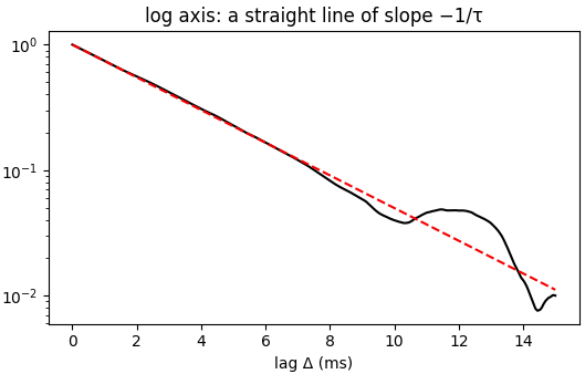
We can determine this time constant in two related ways. Perhaps the most obvious of the two is to measure the autocorrelation of the channel. This autocorrelation will dropoff exponentially with the time constant $\tau$:
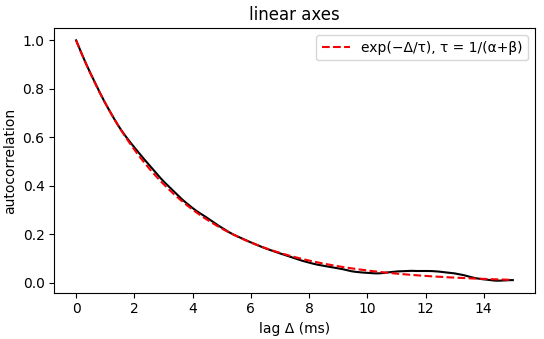
The time constant is even easier to read off when we plot the same relationship on a log-scale:
The second approach is to view the channel fluctuations in the frequency domain. The channel is flickering randomly, so it will contain components at all frequencies. However, the power at each frequency will drop off in a particular way, $$ S(f) = {S_0 \over 1 + (f/f_c)^2}.$$
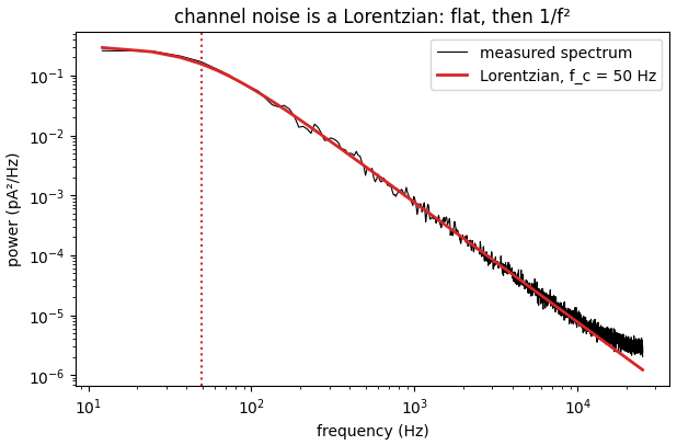
At low frequencies, the power is approximately constant at $S_0$. As frequency increases, power begins to drop off. The frequency at which it drops to $S_0/2$ is the cutoff frequency, $f_c$, and is inversely related to the channel time constant, $$ f_c = {1 \over 2 \pi \tau} = {\alpha + \beta \over 2\pi}.$$
Regardless of how the time constant is computed, with the value in hand, we have $\alpha + \beta$. Since the parabola has given us the other channel parameters $N$ and $i$, we can determine the channel open probability from the mean current $\langle I \rangle $ measured at our holding voltage as $$ p = {\langle I \rangle \over N i} = {\alpha \over \alpha + \beta} = \alpha \tau.$$ Since we also have $\tau$, this equation now gives us $\alpha$. And once we have $\alpha$, $\beta$ is determined as well.
$$\blacksquare$$
Leave a Reply