These are some brief notes on the junction tree algorithm to supplement Section 8.4.6 in PRML.
We’ve seen how to use the sum-product algorithms to do exact marginalization in tree-structured graphs. What if the graph is not tree structured? The junction-tree algorithm converts our general, potentially loopy, graph into a tree, allowing us to run the sum product algorithm. The difference is that the vertices of this new junction tree are no longer single variables, but maximal cliques of a new graph based on our original.
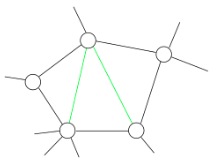
To produce the junction tree, we start with our graph. If it’s a directed graph, we convert it to an undirected graph through moralization. We then triangulate any loops by adding chords, new edges between nodes, so that any loop consisting of 4 or more nodes contains a chord. For example, the original graph below, with edges in black, has been triangulated by adding the green chords:
With our new chordal graph in hand, we apply two theorems.
The first theorem says that chordal graphs can be represented as trees, where the nodes are maximal cliques. Such trees are called clique trees, or junction trees.
Therefore, we find the maximal cliques of our chordal graph. These will take the place of the variable nodes in the sum-product algorithm, except this time each node will potentially represent several variables, all those that belong to a maximal clique.
Just like in the sum-product algorithm, the variable nodes will send messages to each other about the variables they have in common. In ordinary tree-structured graph, there was just one variable that any two nodes had in common. In clique trees, neighbouring nodes can share more than one variable in common. For example, if one clique involves variables $\{A,B,C\}$ and the next $\{B,C,D\}$, then the first will send messages to second about $B$ and $C$.
Now, given our maximal cliques, how do we arrange them into a tree? If we want accurate inference, we can’t do this arbitrarily. We need to ensure that information about variables can be propagated across the tree and doesn’t get “disconnected.”
For example, suppose our cliques were $$C_1 = \{A,B,C\}, \quad C_2 = \{B,C,D\}, \quad C_3 = \{A,C,E\}.$$ Suppose we connected these cliques in the order above, and wanted to compute the marginal value of $C$. The first clique would integrate out $A$ and pass the resulting distribution on $B$ and $C$ to the second clique. That clique would combine the message with its own factor, integrate out $B$ and $D$, and pass the resulting distribution on $C$ to the final clique. That clique would combine the message with its own factor and integrate out $E$ and $A$ to finally produce a value that only depends on $C$.
However, this final value would be incorrect: we marginalized over $A$ twice, once at the beginning and once at the end, and therefore did not correctly account for how $A$ affects the first factor and the last one simultaneously.
Another way to see this to spell out the marginalization our procedure above implies: $$ \sum_{A,E} \phi_3 (A,C,E) \sum_{B,D} \phi_2(B,C,D) \sum_{A} \phi_1(A,B,C).$$ Notice the double marginalization over $A$, at the beginning and at the end.
The problem with our approach above was clearly that $A$ appeared at the beginning, then disappeared, then reappeared at the end. To avoid such situations, we need the running intersection property (RIP). This says that if a variable appears in any two cliques, it should be present in every clique on the (unique) path between them.
A theorem by Jensen then says that if we arrange our cliques so as to produce a maximum spanning tree, the resulting graph will also satisfy the RIP. The weight of an edge between cliques $C_i$ and $C_j$ in the graph is the number of variables they have in common, which we can write as $|C_i \cap C_j|$. The span of the graph is the sum of the weights of all its edges. Therefore, by finding an arrangement of the clique tree that maximizes the span, we’ll also satisfy the RIP.
Returning to our example above, we can compute the span of the faulty arrangement: $C_1 , C_2, C_3$ as $$|C_1 \cap C_2| + |C_2 \cap C_3| = |\{B,C\}| + |\{C\}| = 2 + 1 = 3.$$
In the corrected tree, we reorder the cliques as $C_3, C_1, C_2$. The span of this graph is $$|C_3 \cap C_1| + |C_1 \cap C_2| = |\{A,C\}| + |\{B,C\}| = 2 + 2 = 4,$$ higher indeed than in the previous ordering.
Once we have our clique tree arranged to maximize its span, we assign each of our original factors to exactly one of the cliques. This is possible because the factorization of our original undirected graph was already in terms of cliques. Therefore, each of our factors already belonged to a clique, which was possibly expanded by the triangulation, and will ultimately end up in at least one maximal clique. This is called the family preservation property.
We can then run sum-product as before, except now the messages we pass can involve more than one variable. But it’s fundamentally the same algorithm. And just like when our original graph was a tree, if we run sum product once in the forward direction towards a root, and once backwards, we’ll have all the messages we need to compute all the marginals in the graph.
So what’s the catch? The clique sizes. The vertices in our graph are now cliques, and the marginalizations are exponentially expensive in the clique sizes. In a tree, all cliques are of size 2, so we’re ever only integrating over one variable to compute messages. In a general graph, the cliques can be larger, and the computational cost will rise exponentially.
Summary
To sum up, we can run exact inference in arbitrary graphs by first turning them into (clique) trees, as follows:
- Make a directed graph undirected by moralization.
- Triangulate all cycles.
- Identify the maximal cliques.
- Find a maximum spanning subtree.
- Assign each factors to one maximal clique.
- Perform sum-product with the clique containing the variable(s) of interest as the root.
$$\blacksquare$$
Leave a Reply