These are my notes on the Ito calculus as presented in Chapter 8 of Potter’s “A First Course in Random Matrix Theory.” I follow that chapter pretty closely, filling in some of the gaps in the presentation as I go.
Brownian Motion
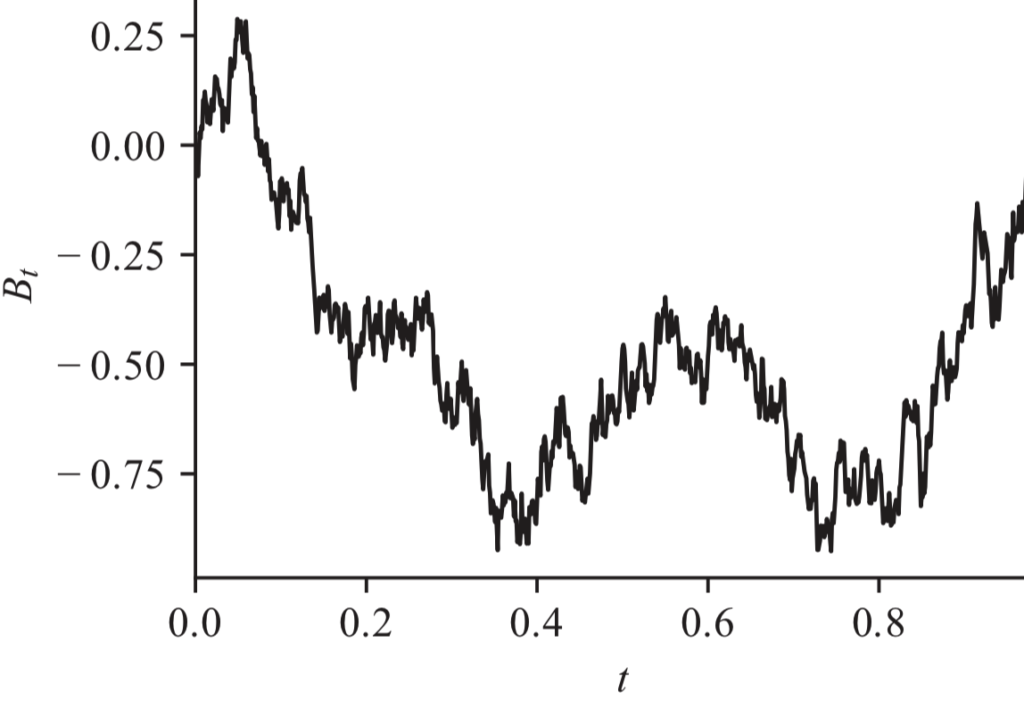
We start with Brownian motion process, $X_t$. This has drift $\mu$, and diffusion variance $\sigma^2$, so, $$ X_t \sim \mathcal{N}(\mu t, \sigma^2 t).$$
The Normal distribution is infinitely divisible. This means we can break a variable distributed that way into a sum of independent contributions.
This is intuitive for our variable above. We can think of its overall position $X_t$ as the sum of infinitesimal motions up to that point. In fact, that’s how the Brownian motion was originally observed, the result of countless random, independent perturbations, of e.g. dust particles under a microscope.
To formalize this, we split the time interval $[0,t]$ into $N$ sections. We can now think of $X_t$ as the sum of perturbations in each interval: $$X_t = \sum_{k=0}^{N-1} \delta X_k.$$
Each perturbation will contribute its own portion of drift and diffusion, $$ \delta X_k \sim \mathcal{N}(\mu \delta t, \sigma^2 \delta t).$$ We can write this more suggestively as $$ \delta X_k = \mu \delta t + \sigma \mathcal{N}(0, \delta t).$$ This equation makes it clear that each contribution has a non-random part, the drift, and a random diffusive part.
If we take the limit as $\delta t \to 0$, we get $$ dX_t = \mu dt + \sigma dB_t,$$ where $dB_t$ is a centered, infinitesimal Gaussian perturbation
One subtlety that’s crucial to Ito’s approach is exactly when the perturbations are supposed to arrive. Ito assumes that the perturbations arrive at the beginning of the interval. This then means that the the perturbation at $t$ will be independent of the value $X_t$ before it. This is called Ito’s prescription.
Transforming by a function
Now what happens when we transform through a function? Let’s apply a Taylor expansion to second order:
$$dF = F(X + dX) – F(X) = F'(X) dX + {F^{”}(X) \over 2} dX^2.$$
$$F'(X) dX = F'(X) (\mu\, dt + \sigma dB_t).$$
$$ dX^2 = \mu^2 dt^2 + \sigma^2 dB_t^2 + 2 \mu \sigma^2 dB_t dt.$$
If we expand this out as
$$ dX^2 = \mu^2 dt^2 + \left(\sigma^2 dB_t^2 – \sigma^2 dt\right) + \sigma^2 dt + 2 \mu \sigma^2 dB_t dt.$$
The first term is $O(dt^2)$, the last term is $O(dt^{3/2})$. The second term has mean 0, but turns out to be of order $dt$, so we can’t ignore it in isolation. But we’ll be integrating such terms, and they’re all uncorrelated, so Ito showed that we can ignore them in the integration.
So, as long as we agree that we’re going to be integrating things, we end up with $$ dX^2 \to \sigma^2 dt,$$ and our differential becomes $$ dF = F'(X) dX + \underbrace{{\sigma^2 \over 2} F^{\prime\prime}(X) dt}_{\text{Ito correction}}.$$ Notice the Ito correction relative to the ordinary (non-stochastic) case.
Example: Variance of Brownian Noise
Suppose we have a driftless Brownian noise process, $$ dX_t = \sigma dB_t.$$
We expect the variances of $X_t$ to be $\sigma^2 t$. Let’s see if we can derive that.
The variance of $X_t$ is $$\var(X_t) = \EE X_t^2 – (\EE X_t)^2 = \EE X_t^2.$$
So if we take $F(X) = X^2$, then $$ \var(X_t) = \EE F(X_t).$$
Using Ito’s formula above, $$ dF_t = F'(X_t) dX_t + {\sigma^2 \over 2}F^{”}(X_t) dt = 2X_t dX_t + \sigma^2 dt = 2\sigma X_t dB_t + \sigma^2 dt.$$
We then get $$F_T = \int_0^T 2\sigma X_t dB_t + \sigma^2 dt.$$
By Ito’s prescription, $dB_t$ is independent of $X_t$, so the first term integrates to zero, though it presumably has some fluctuations.
The second term gives $\sigma^2 T.$
So, $ \EE F_T = \sigma^2 T,$ as expected.
The Langevin Equation
To motivate the Langevin equation, let’s start with a process with increments are $$ dX_t = dB_t + F(X_t) dt.$$ This is a combination of Brownian motion with a perturbing force. Brownian motion will increase variance with time. This gives us variability that we can sculpt to produce various effects.
We might be interested in:
- The stationary distribution of $X_t$, if one exists.
- Setting $F$ to achieve a desired stationary distribution.
- Sampling $X_t$ as a means of sampling from some target distribution.
- Computing averages against the target distribution empirically using the samples.
It will be useful to parameterize $F(X_t)$ as the gradient of some potential, so $$ F(X_t) = -{1 \over 2} V'(X_t).$$
Now let’s see what happens if we compute some function $f$ of the particle. From Ito’s formula, we have
\begin{align*} df(X_t) &= f'(X) dX + {1 \over 2}f^{”}(X) dt\\ &= f'(X) dB_t – {1 \over 2} f'(X) V'(X) dt + {1 \over 2} f^{”}(X) dt \end{align*}
Taking expectations relative to the assumed stationary distribution $P(x)$ on both sides, $$ \EE df(X_t) = \EE f'(X) dB_t – {1 \over 2} \EE f’ V’ dt + {1\over 2} \EE f^{”} dt.$$
At stationarity, we’ll assume that $df/dt$ doesn’t change in expectation, so the first term is zero.
The second term is zero by Ito’s prescription. So we get $$ \boxed{\EE (f'(X) V'(X)) = \EE f^{”}(X).}$$
This is an interesting expression itself, and says that we can compute the expectation of the second derivative of any $f$ by averaging its first derivative against $V'(X)$.
Expanding out the expressions, we get $$ \int f'(X) V'(X) p(X) dX = \int f^{”}(X) p(X) dX.$$
At this point, we want to re-express the right-hand side. Since $$ d (f'(x) p(x)) =f^{”} p(x) dx + f'(x) p'(x),$$ if we integrate over the whole domain, we get $$ \left. f'(x) p(x) \right|_{-\infty}^\infty = \int f^{”} p(x) dx + \int f'(x) p'(x) dx.$$
If $f$ and $p$ are well behaved, then since $p(x)$ integrates to 1, it must go to 0 at either extreme, so we get $$ \int f^{”} p(x) dx = – \int f'(x) p'(x) dx.$$
Substituting that into our expression above, we get $$ \int f'(X) V'(X) p(X) dX = -\int f'(X) p'(X) dX.$$
Since this must be true for any $f(X)$, we get $$ V'(X) p(X) = – p'(X) \implies V'(X) = – {p'(X) \over p(X)} = – {d \log p(X) \over dX}.$$ So we arrive at $$ V(X) = – \log p(X) + \text{const},$$ or $$ p(X) = {1 \over Z} e^{-V(X)}.$$
So what this says is that if we have a stochastic process whose increments are $$\boxed{ dX_t = dB_t – {1 \over 2} V'(X_t) dt,}$$ so noisy gradient descent, then its stationary distribution will be the one given above. This is the Langevin equation.
An application to neural coding
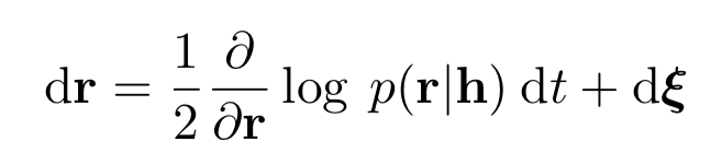
The dynamics above can be used to show how neurons can perform inference. Setting $V(X)$ be the negative log posterior conditioned on some observations, neurons performing gradient ascent on that posterior, while subject to Brownian noise, would, asymptotically, generate samples from the posterior. For example, see this paper by Hennequin et al., where they start their analysis by considering dynamics of the form
The Ohrstein-Uhlenbeck Process
As an example we can determine the process whose stationary distribution is the standard Gaussian. In that case, $V(X) = X^2/2$, so $$ dX_t = dB_t – {1 \over 2} V'(X_t) = dB_t – {1 \over 2} X_t.$$ This is the Ohrstein-Uhlenbeck process.
Another way to derive this process is to return to Brownian motion and notice that the variance there increases with time. My naive approach would have been to take the Brownian motion and scale it by a factor of $\sqrt{t}$. This would have produced a process with constant variance, but it
- Requires knowing $t$.
- Blows up at $t = 0$.
Instead of applying such a global shrinkage, we can apply it locally, at each increment. In particular, we can say $$ X_{t+ dt} = {X_t \over \sqrt{1 + dt}} + dB_t.$$
To see that this does the right thing, we can track the variance: $$ \var(X_{t+dt}) = {\var(X_t) \over 1 + dt} + dt, $$ so $$ \var(X_{t+dt})(1 + dt) = \var(X_t) + dt +dt^2.$$ Dropping the $dt^2$ term and rearranging, $$ {\var(X_{t+dt}) – \var(X_t) \over dt} = 1 – \var(X_{t+dt}),$$ which goes to $$ {d\var(X)\over dt} = 1 – \var(X).$$ So the variance decays to unity, as desired.
Example: Student’s t-Distribution
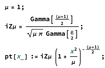
The Student’s t-distribution can be parameterized as

The potential for this distribution satisfies $$ V(x) = – \log P + \text{const} = {\mu + 1 \over 2} \log \left(1 + {x^2 \over \mu}\right).$$
To determine the process that produces the above as its stationary distribution, we take the derivative of the potential, $$ V'(x) = {\mu + 1 \over 2} {\mu \over \mu + x^2} {2 x \over \mu} = {\mu + 1 \over \mu + x^2} x.$$
From this we get $$ dX_t = dB_t – {1 \over 2} {\mu + 1 \over \mu + X_t^2} X_t.$$
When $X_t$ is small, this behaves like an OU process, $$ dX_t \approx dB_t – {1 \over 2}{\mu +1 \over \mu}X_t.$$ Actually, the restoring force is stronger than in the O-U process, so it pulls values towards zero more strongly.
However, when $X_t$ is large, the corrective deviations are much smaller than for the OU process: $$ dX_t \approx dB_t – {1 \over 2}{\mu+1 \over X_t^2} X_t =dB_t – {1 \over 2}{\mu+1 \over X_t}.$$ In fact, the larger $X$ gets, the free-er the diffusion becomes.
Note also that as $\mu \to \infty$, the process approaches an OU process, which reflects how the corresponding Student’s t-distribution approaches the Gaussian.
Simulations
OU Process
First, let’s generate an OU process. Below I specify two functions for doing this: one that takes the increments perspective, and the other that takes the shrinkage one:

We can sample a million points from each, dropping the first 1000 for burn in:

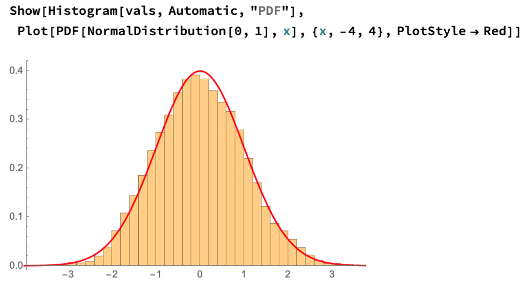
Overlaying the standard normal on the histogram of samples shows good agreement:
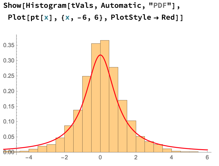
Student’s t-Distribution
First we’ll set up the target distribution and its PDF:
Next we’ll set up the increments:

Next we’ll generate the samples. We don’t sample in one run, since the samples get stuck around high values. This is easy to understand from our discussion of how the increments behave, and how they get smaller when the values get larger.
Instead, we’ll do a bunch of runs from random starting positions, and pool the results:

Plotting the desired distribution over the histogram shows good agreement:
Fokker-Planck Equation
We can also follow how the probability distribution $P$ itself evolves with time.
We start with our process $$dX_t = dB_t + F(X_t) dt,$$
and take some arbitrary well-behaved function $f$ and apply Ito’s formula to study its increments: $$ df(X_t) = f'(X_t) dX_t + {1 \over 2}f^{”} dt = f'(X_t) dB_t + f'(X_t) F(X_t) dt + {1 \over 2} f^{”} dt.$$
Taking expectations of this, $$ \EE df(X_t) = d\EE f(X_t) = \EE f'(X_t) dB_t + \EE f'(X_t) F(X_t) dt + {1 \over 2} \EE f^{”} dt.$$
By Ito’s prescription the first term on the right-hand side is zero, so we get $$ d\EE f(X_t) = \EE f'(X_t) F(X_t) dt + {1 \over 2} \EE f^{”} dt.$$
Dividing out by $dt$ we get \begin{align*} {d\EE f(X_t) \over dt} &= {d \over dt} \int f(X) P(X, t) dx\\ &= \int f(X) {\partial P(X,t) \over \partial t} dx = \int f'(X) F(X) P(X,t) dx + {1 \over 2}\int f^{”}(X) P(X,t) dx.\end{align*}
Applying integration by parts once to the first term, and twice to the second term, and using the boundary conditons on $P$ whereby it and its first derivative go to zero at infinity, we get $$ \int f(X) {\partial P(X,t) \over \partial t} dx = -\int f(X) {\partial F(X) P(X,t) \over \partial X} dx + {1 \over 2}\int f(X){\partial^2 P(X,t) \over \partial X^2} dx.$$
Since this must be true for any $f(X)$, we get the Fokker-Planck equation
$$ \boxed{ {\partial P(X,t) \over \partial{t}} = – {\partial F(X) P(X,t) \over \partial X} + {1 \over 2}{\partial^2 P(X,t) \over \partial X^2}.}$$
Example: OU Process
Let’s check this equation for the OU process. For that process, $F(X) = -X/2$. At stationarity, we should get from the above that $$ -{\partial X P(X,t=\infty) \over \partial X} = {\partial^2 P(X,t=\infty) \over \partial X^2}.$$
For the standard Gaussian, $ P'(X) = -X P(X),$ so we see that this equation holds.
$$\blacksquare$$
Leave a Reply