In Harris et al. the authors study how the decoding weights that read out the identity of the odour stimuli from neural activity change over time. To describe these changes, the Mihaly has developed a parsimonious model called the “Drift Decoder”, which models the weights as the sum of an initial value, plus a temporal sequence of rank-1 modes: $$ \WW(t) = \WW_0 + \sum_{k = 1}^K \WW_k \alpha_k(t).$$ Here each of the added modes $\WW_k$ is rank-1, and the activation terms $\alpha_k$ are assumed to be sigmoidal, with their onset times and slopes being fitted to the data. With this model, the authors able to study the changes in weights that occur due to task demands and behavioural states, for example during sleep.
Notice that if all the modes were active all the time, then this model, using orthogonal rank-1 modes, would be finding the SVD of the residuals after subtracting $\WW_0$. These modes would be temporally global, defined over the entire duration of the data. What’s interesting about the Drift Decoder is that the sigmoidal activations makes the learned modes temporally local. For example, the first mode captures the variance in the first chunk of the data, the second mode captures the additional variance introduced in the next chunk of the data, and so on. The resulting modes therefore capture how the data is changing, rather than its global properties.
The Drift Decoder fits the sigmoids directly. In the model below, I try to give a generative basis to the Drift Decoder by modeling the sigmoids are readouts of and underlying linear, sequential dynamics. This can perhaps give additional insight to the physical processes generating the observations.
Model
Our model is
\begin{align*} \xx_{t} &= \mathbf{L} \xx_{t-1} + \bb + \boldsymbol{\eta}_t, & \boldsymbol{\eta}_t & \sim N(0, \boldsymbol{\beta}_x^2)\\ \zz_{t} &= \sigma(\xx_{t})\\ \yy_{t} &= \CC \zz_{t} + \dd + \boldsymbol{\epsilon}_t, &\boldsymbol{\epsilon}_t & \sim N(0, \boldsymbol{\beta}_y^2), \end{align*} where $$\sigma(x) = {1 \over 1 + e^{-x}}$$ is the standard sigmoid, and is applied element-wise to its arguments.
The name
When the dynamics $\LL$, and the inputs $\bb$ are $\bzero$ and the latent noise has unit variances, the latents become iid random samples from the standard Gaussian. If we then replace the sigmoid nonlinearity with just linear activations, the model reduces to Factor Analysis. I’ve hence named the model Sequential Sigmoidal Factor Analysis. To see what makes it sequential, see the next section.
Sequential Activation
The lower triangular structure of $\LL$ encourages sequential activation. We will first demonstrate sequential activation analytically in a toy example, before demonstrating it numerically in a larger example.
Toy Example
1-D case
We will first demonstrate how the parameters determine the sigmoidal activation properties of a single unit.
In the one-dimensional case, $$ x_{n+1} = a x_n + b, \quad z_n = \sigma(x_n), \quad z_n \ \sigma(x_n), \quad 0 < a < 1.$$
Asymptotic activation. The solution at time $n$ is $$x_n = a^n x_0 + b { 1 – a^n \over 1 – a} \to x_\infty \triangleq {b \over 1 – a}.$$ The exact value of this asymptotic drive is not important, as long as it’s large enough to saturate the sigmoid, activating the corresponding mode.
Onset time. We will initialize $x(0) \ll 0$ so that the sigmoid starts in the off state. If $b>0$, then the sigmoid will eventually turn on. We can define the activation time as when the sigmoidal output crosses $1/2$, equivalently when the drive crosses 0: $$ a^n x_0 = b {a^n – 1 \over 1 – a} \implies a^n (b – x_0) = {b \over 1 – a} \implies n = {1 \over \log a}\log{x_\infty \over b – x_0} \triangleq t_\text{on}.$$
Onset speed. We can measure the speed of activation by the slope of the sigmoid when it crosses $1/2$. At that point the drive is 0, so at the subsequent time step, the drive will have a value of $b$, which we can take as the derivative of the drive. $$ {dz(x(t)) \over dt} = {dz\over dx}{dx \over dt} = {1 \over 4} b.$$
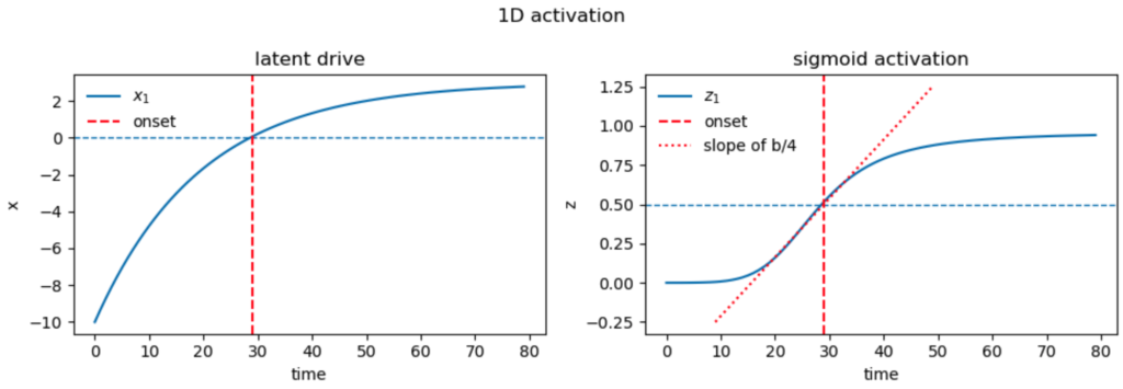
Thus, with the three parameters of initial condition $x_0$, self-excitation $a$, and drive $b$, we can determine the three desired properties of onset-time, onset-slope, and asymptotic activation. We show an example of this below for $a = 0.95$, $b = 0.15$, initialized to $x[0] = -10$.
2-D Example
We now demonstrate sequential activation in a 2-dimensional case. The dynamics are $$ \xx_{n+1} = \begin{bmatrix}a & 0 \\ s & a \end{bmatrix} \xx_n + \begin{bmatrix}b_1 \\ b_2 \end{bmatrix}, \quad \zz = \sigma(\xx).$$ The new parameter $s$ controls the drive from the first latent to the second. The element-wise dynamics are \begin{align*} x_{1,n+1} &= a x_{1,n} + b_1 \\ x_{2,n+1} &= a x_{2,n} + s x_{1,n} + b_2. \end{align*}
The dynamics of the first unit are just as in the previous section. Those of the second are exponential decay of the initial condition, plus convolution with the input from the first unit on top of its own drive: $$ x_{2,n} = a^n x_{2,0} + \sum_{k=0}^{n-1}a^{n -1 -k} (s x_{1,k} + b_2).$$
Expanding this out, we get $$ x_{2,n} = a^n x_{2,0} + n s a^{n-1} x_{1,0} + b_2{1 – a^n \over 1 – a} + s b_1 {1 – n a^{n-1} + (n-1) a^n \over (1 – a)^2}.$$
Asymptotic activation. From the expression above we get the asymptotic activation of the second unit as $$ x_{2, \infty} = {b_2 \over 1 – a} + { s b_1 \over (1 – a)^2} = {s x_{1, \infty} + b_2 \over 1 – a}.$$ In other words, the asymptotic activation of the second unit is what would be determined by its own drive $b_2$, augmented by the activation of the first unit.
Enforcing sequential activation. Note also that by setting $b_2 < 0$, we can ensure that the second unit does not activate without driver from the first.
Onset time. There isn’t a simple closed-form expression for onset-time. We can simply define it as the minimum index at which the latent exceeds 0.
Onset speed. Given the onset time $n^*$, we compute the slope of the latent activation as $$x_{2,n^*+1} – x_{2,n^*} = (a – 1) x_{2,n^*} + s x_{1,n^*} + b_2.$$ Since at the onset $x_{2,n^*} \approx 0,$ we get $$ \Delta x_{2,n^*} \approx s x_{1, n^*} + b_2.$$ Hence, the slope of the sigmoid is $$ \Delta z_{2,n^*} = \sigma'(0) (s x_{1,n^*} + b_2) = {1 \over 4}(s x_{1, n^*} + b_2).$$ Like the asymptotic activation, this expression is just like its counterpart for the first unit, but augmented by drive from that unit.
Although the dependencies of our three observable properties on the parameters are more complex for the second unit than for the first, note that we also have three new degrees of freedom: the initial condition $x_{2,0}$, the self-excitation $b_2$, and the upstream excitation $s$. Therefore, we expect to have enough parameters to fit the observable properties numerically.
Below we demonstrate numerical activation of two modes. The parameters of the first latent remain as before. The parameters of the second are $b_2 = -0.05,$ $x_2[0] = -11$, and the strength of the drive from the first unit is $s = 0.08$.
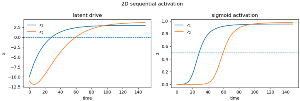
Notice that the self-drive of the second unit negative, so it would be unable to activate without help from the first unit. This is visible in the initial downward dip of $x_2$ (left panel, orange curve).
Large Example
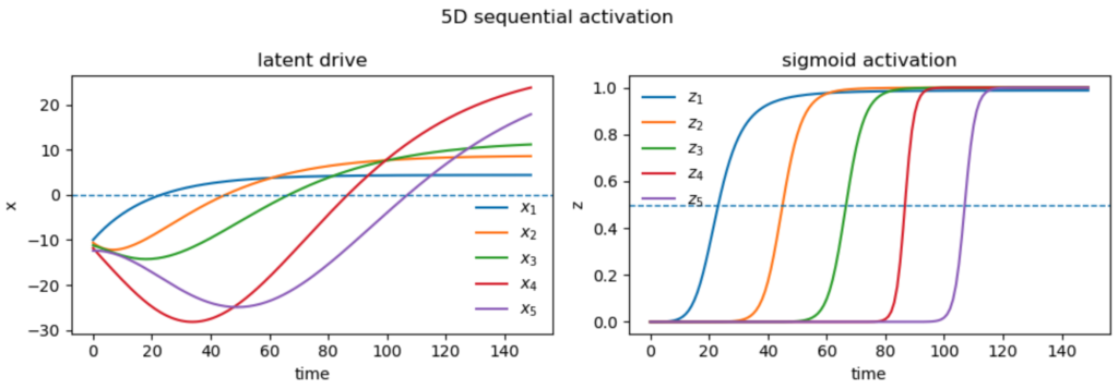
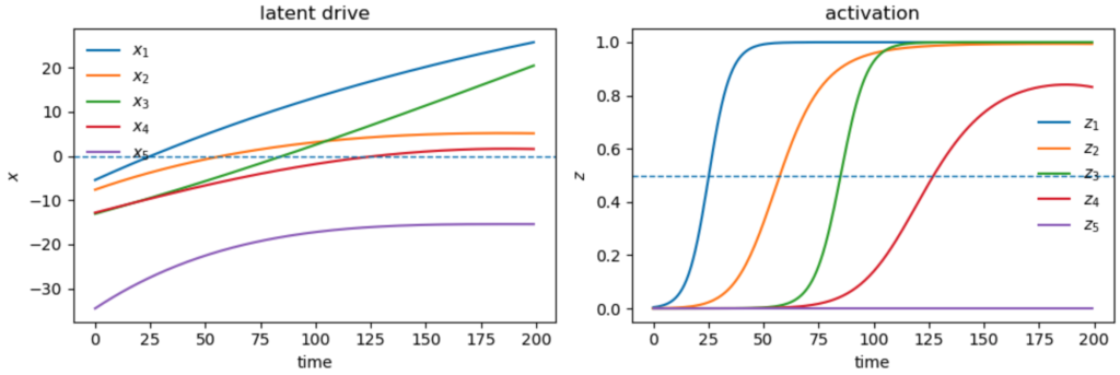
We can naturally extend our approach to more latents. At each stage, three new parameters are introduced, which can be adjusted to match the three desired properties of the new latent. Below we show an example with 5 latents
Sequences without Sequencing
If all we care about is the cross-over time and cross-over slopes of the latents, ChatGPT pointed out a trivial solution which doesn’t require interaction between the modes. We can set $\LL$ to zero, making the drives $x_i$ independent and linear in time. We just set their inputs $b_i$ to the desired slope, and their initial conditions to match the desired offset: $$ x_i(t) = b_i (t – t_{\text{on}, i}) = b_i t + x_i(0), \quad x_i(0) \triangleq – b_i t_{\text{on}}. $$ Thus there is no explicit sequencing that happens here, no drive of one unit activating that of the next. The units are independent, and just happen to activate sequentially. Here is an example:
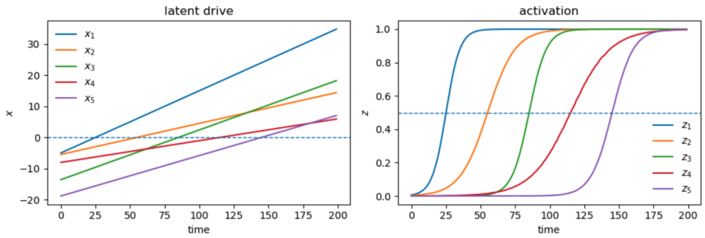
Such solutions may give the desired mode activations $z_i$, but the behaviour of the drives $x_i$ might not be plausible. For example, in the neural data of Harris et al., it may not be plausible to believe that the the drives producing the mode activations are receiving constant positive input throughout to produce the sequencing behaviour, or that they have vastly different initial conditions. To achieve more realistic latent behaviour, it may be necessary to impose further conditions, such as all modes having the same initial conditions, or the inputs to each mode except the first being negative, to encourage the emergence of sequential activation.
Fitting to Data
Parameter counts
Our latent dynamics are $$ \xx_{n+1} = \begin{bmatrix} a & 0 & 0 & \dots & 0 \\ s_1 & a & 0 & \dots & 0 \\ s_2 & s_1 & a & \dots & 0 \\ \vdots & \vdots & \vdots & \ddots & \vdots \\ s_{K-1}, & s_{K-2}, & s_{K-3} & \dots & a \end{bmatrix} \xx_n + \bb + \boldsymbol{\eta}_n$$ Thus, our transition matrix $\LL$ is constrained to have the same parameters below every diagonal. This implies a symmetry in the dynamics: each latent drives those downstream in the same way. Therefore, the transition matrix only requires $K$ parameters, instead of the $K(K+1)/2$ required for a generic lower-triangular matrix.
We saw above that to specify asymptotic activation values, onset times, and onset speeds, we also need to specify drives and initial conditions per unit, contributing $2K$ parameters. We also allow each unit to have its own latent-space noise variance, contributing a further $K$ parameters.
Therefore, our latent dynamics require $4K$ parameters.
The observations are linear in the sigmoidal latents, plus observation noise $$ \yy_t = \CC \zz_t + \boldsymbol{\epsilon}_t.$$ The observation matrix $\CC$ contributes $N K$ parameters, and the channel specific noise variances a further $N$.
Therefore, our observation model requires $ N(K+1)$ parameters.
In total, our model thus requires $ 4K + N(K+1) $ parameters, and is therefore linear in both the number of observation channels, and the latent-space dimension.
These numbers can be further reduced, for example by enforcing the same noise variance across latents, or across observations. The largest contribution to the parameter counts is from the observation matrix, and this can be reduced by parameterization. For example, in the Drift Decoder, the observations correspond to vectorized weight matrices, requiring $m_1 m_2$ elements to be fit, where $m_1$ and $m_2$ are the dimensions of the weight matrix. However, by parameterizing the components of the observation model as rank-1 matrices, the number of parameters is reduced to a factor of $m_1 + m_2$.
Fitting
We fit the parameters and latents using least squares.
Initialization
Initialization is important to get good solutions. We initialize the data to a sequential solution by splitting the data into $K+1$ consecutive blocks of equal size, and requiring that the modes activate in sequence at each interior boundary between the blocks. That is, for $K$ modes to explain data of length $T$, we requires $z_n(n T/K) = 0.5$. We set the required slopes at activation to a constant value, typically 0.2. We then use the “trivial” linear solution described above to determine the latent drives, and therefore the initial conditions.
Initializing the model is important for finding good solutions. Since the observations are $$ \yy_t = \CC \zz_t + \dd,$$ and the modes evolve from 0 to 1, we initialize at a sequential solution by splitting the data into $K + 1$ consecutive temporal blocks. In the first block, all the modes are assumed off, leaving only $\dd$ to explain the responses. We therefore set the value of $\dd$ to the average value of the observations in the first block. We set the self-excitation value, $a_i$, of each mode to value near 1, and the lateral excitation values to 0.
Performing the fits
Once the sigmoidal activations are known, the observation parameters $\CC$ and $\dd$ can be determined by least squares. We compute the residuals between the predictions and observations and use nonlinear-least squares to adjust the parameters of the latent dynamics to improve the fit.
Boundary Conditions
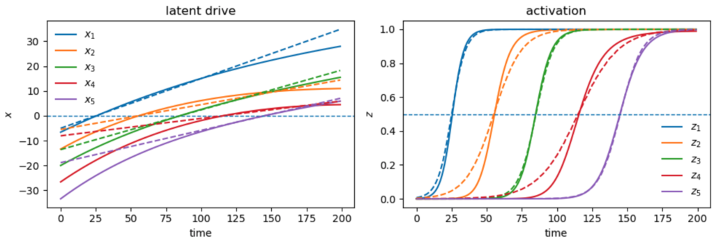
We found that multiple solutions can explain the same set of observations. In the example below, one of the latents, $z_4$ does not fully activate, and in fact is diminishing towards the end of the data.
To avoid such solutions, we impose bondary condtions on the latent drives $x_i$ that encourage values below a certain margin at the start of the data, and above a certain margin at the end. This in turn encourages the latents to all start near 0, and end near 1, producing more realistic fits. The example below demonstrates this, with the true values of the latents given in dashes:
Fitting Neural Data
To be inserted…
Conclusions
To be determined…
$$\blacksquare$$
Leave a Reply