Below are notes on Saxe et al.’s “A mathematical theory of semantic development in deep neural networks.” that I initially made for the Discord sessions of March 2026, and which I’ve now (5 May 2026) finalized after presenting the paper at the Crick.
In this paper the authors use a two-layer linear network to investigate how brains and machines uncover structure in data. Specifically, they consider a problem of mapping items, modelled on plants and animals, to their features, where features exhibit hierarchical structure, ranging from high-level features like “can move” to low-level features like “has leaves”. Agents in the world encounter items and observe their features. The question is whether and how such agents can organize these observations to reflect the underlying structures that they reflect.
I think this is a great paper for at least four reasons. The first is scientific, and the remaining three are meta-scientific
- The scientific contribution: it gives us a concrete framework for understanding semantic development and answering various questions about it.
- Simplicity: Rather than studying semantic development by throwing large datasets at fancy deep learning models, the authors study a very simplified version of the problem, which they can analyze in detail to get insight.
- Theoretical moves: Despite the simplicity of their model, it still starts off as being hard to analyze. Through a series of assumptions they simplify the model to something that has a closed form solution. Remarkably this solution well describes the behaviour of the model before simplifications.
- Picking a good title: It doesn’t matter if you have the best idea in the world, it won’t matter if nobody reads it. They could have called their paper something cryptic “Two-layer linear networks perform sequential SVD”, which is the core of their findings, but that would sound too technical to most people, even if they’d benefit from reading it. Instead, they refer to “deep neural networks”, even though the network is only two layers deep, and is linear. Neverthless, their insights apply to deeper, nonlinear networks, and so by using a good title they can spread knowledge of their results more effectively. For an example of a poor title, see this paper.
The paper has two parts. The first part is about learning. The second part is about what is learned, the SVD of the input output covariance, and how the resulting bases are useful for answering a variety of questions. In this post I’ll focus on the first part.
Problem Setup
The learning problem they study is mapping items such as different plants and animals, to various properties, such as whether they can move, whether they are big, etc.
Semantic development
Deep nonlinear networks solving this task can produce a hierarchical decomposition in time: early in learning the representation of all items are similar. As learning progresses, items become gradually distinguished, first along high-level dimensions, later along more fine-grained distinctions. Below is a panel showing dimensions-reduced representations for one such network:
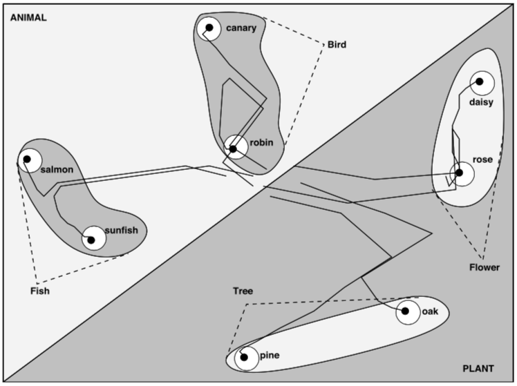
The representations for the items seem to first split by the animal/plant distinction, then by the e.g. bird/fish distinction, till finally they arrive at their specific instance. This seems qualitatively similar to what happens in human learning, where (presumably) broad categories are learned before narrow distinctions. How does this come about?
A deep linear network
To address this problem while retaining analytic tractability, the authors turn to a deep linear network. It’s deep because it has one hidden layer, and linear because the activations of all units are linear. Depth doesn’t add anything to the network’s input-output transformation, but, as it turns out, creates interesting learning dynamics.
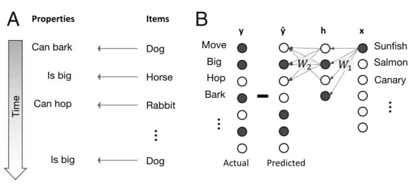
They encode inputs $\xx$ as one-hot vectors indicating specific animals, plants etc. Target outputs are binary vectors $\yy$ indicating various properties of each input. Their predicted output is generated by transforming the inputs to a hidden layer via a first set of weights $\WW_1$, and then transforming the hidden layer activations to predicted outputs $\hat \yy$ using a second set of weights $\WW_2$: $$ \hat \yy = \WW_2 \hh , \quad \hh = \WW_1 \xx.$$
Learning is performed by minimizing the least-squares loss $$L = {1 \over 2}\|\yy – \hat \yy\|_2^2.$$ Item-property pairs $(\xx_i, \yy_i)$ are presented in sequence, and weights are updated down the loss gradient after each such presentations.
Weight updates by gradient descent
To find the gradients, we compute the differential $$ dL = -\bE^T d\WW_2 \WW_1 \xx – \bE^T \WW_2 d\WW_1 \xx,$$ where we’ve defined $$ \bE \triangleq (\yy – \hat \yy) = (\yy – \WW_2 \WW_1 \xx).$$
The gradients are then $${ \partial L \over \partial \WW_1} = -\WW_2^T \bE \xx^T = -\WW_2^T(\yy- \WW_2 \WW_1 \xx) \xx^T,$$ and $${\partial L \over \partial \WW_2} = -\bE \xx^T \WW_1^T = -(\yy – \WW_2 \WW_1 \xx) \xx^T \WW_1^T.$$
The weight updates are a stepsize $\lambda$ down these gradients: \begin{align*} \Delta \WW_1 &= -\lambda {\partial L \over \partial \WW_1} = -\lambda \WW_2^T(\yy- \WW_2 \WW_1 \xx) \xx^T \\ \Delta \WW_2 &= -\lambda {\partial L \over \partial \WW_2} = -\lambda (\yy- \WW_2 \WW_1 \xx) \xx^T \WW_1^T \end{align*}
From discrete to continuous time
To convert these discrete, per-item, updates into continuous time dynamics, we can take the changes above to occur over a time step $\Delta t$, and consider the net change after having viewed all $P$ items in the dataset.
For the first set of weights, this would look like \begin{align*} \Delta \WW_1 &= \Delta t \lambda \sum_{i=1}^P \WW_2^T(\yy_i- \WW_2 \WW_1 \xx_i) \xx_i^T\\ &= \Delta t \lambda \WW_2^T \left(\left(\sum_{i=1}^P \yy_i \xx_i^T\right)- \WW_2 \WW_1 \left(\sum_{i=1}^P \xx_i \xx_i^T\right)\right) \\ &= \Delta t \lambda P \WW_2^T (\Sigma_{yx} – \WW_2 \WW_1 \Sigma_x), \end{align*} where we’ve defined the covariances $$ {1 \over P} \sum_{i=1}^P \yy_i \xx_i^T = \Sigma_{yx}, \quad {1 \over P}\sum_{i=1}^P \xx_i \xx_i^T = \Sigma_x.$$
Then $$\lim_{\Delta t \to 0} {1 \over P \lambda}{ \Delta \WW_1 \over \Delta t} = \tau {d \WW_1 \over dt} = \WW_2^T (\Sigma_{yx} – \WW_2 \WW_1 \Sigma_x),$$ where we’ve defined $\tau \triangleq {1/P\lambda}$.
Similarly, for the second set of weights, we get $$ \tau {d \WW_2 \over dt} = (\Sigma_{yx} – \WW_2 \WW_1 \Sigma_x) \WW_1^T.$$
Weight dynamics
At this point we have the following analyze: \begin{align*} \tau {d \WW_1 \over dt} &= \WW_2^T (\Sigma_{yx} – \WW_2 \WW_1 \Sigma_x) \WW_1^T\\ \tau {d \WW_2 \over dt} &= (\Sigma_{yx} – \WW_2 \WW_1 \Sigma_x) \WW_1^T. \end{align*} So, despite our simple, linear model of a two layer network, the learning dynamics are coupled, and non-linear, since $\WW_2$ and $\WW_1$ multiply in the expressions above.
Instead of using advanced math to perform a complicated analysis of the equations above, the authors apply George Polya’s advice that when one encounters a problem one can’t solve, one should try solving a simpler problem that can be solved. They will now apply a series of approximations and assumptions, that I’ll call moves, to convert the system above into one that has a closed-form solution.
First Move: Decorrelated Inputs
The dynamics above depend on both the input covariance $\Sigma_x$, and the input-output covariance $\Sigma_{xy}$.
To gain insight into the weight dynamics, we can first simplify the problem by assuming that the input dimension are uncorrelated, so $ \Sigma_x = \II$.
Second Move: Switching coordinates
We can then switch to coordinates that reflect the input and output statistics, by applying SVD to the input-output covariance, $$\Sigma_{yx} = \UU \SS \VV^T,$$
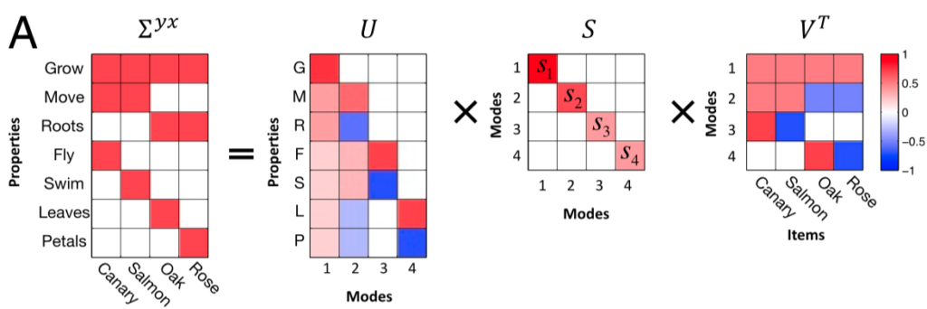
The rows of $\VV^T$ form an orthonormal basis for the input, and those of $\UU$ do the same for the output. Since the weights combine as $\WW_2 \WW_1$ to transform the inputs to the outputs, we can reparameterize the weights in terms of the $\UU$ and $\VV$ and an arbitrary orthogonal matrix $\RR$ as $$ \WW_1 = \RR \ol{\WW}_1 \VV^T, \quad \WW_2 = \UU \ol{\WW}_2 \RR^{T}.$$
We can express the dynamics in terms of this parameterization as \begin{align*} {d \WW_1 \over dt} &= \RR {d \ol{\WW_1} \over dt} \VV^T \\ \implies {d \ol \WW_1 \over dt} &= \RR^T {d \WW_1 \over dt} \VV\\ &= \RR^T\WW_2^T (\Sigma_{yx} – \WW_2 \WW_1 ) \VV \\ &= \RR^T \RR \ol{\WW}^T_2 \UU^T(\UU \SS \VV^T – \UU \ol{\WW}_2 \RR^T \RR \ol{\WW}_1\VV^T)\VV \\ &= \ol{\WW}_2 ^T( \SS – \ol{\WW}_2 \ol{\WW}_1). \end{align*}
Similarly, $$ {d \ol{\WW}_2 \over dt} = (\SS – \ol{\WW}_2 \ol{\WW}_1)\ol{\WW}_1^T.$$
Third Move: Diagonal Assumption
To further simplify the analysis, they now assume that $\ol{\WW}_1$ and $\ol{\WW}_2$ are diagonal, with elements $c_\alpha$ and $d_\alpha$ respectively. This makes the dynamics above decouple into \begin{align*} {d c_\alpha \over dt} &= (s_\alpha – c_\alpha d_\alpha) d_\alpha \\ {d d_\alpha \over dt} &= (s_\alpha – c_\alpha d_\alpha) c_\alpha \end{align*}
The dynamics of the net transformation $\WW_2 \WW_1$ in the transformed coordinates are then captured by the dynamics of the product $\ol{\WW}_2 \ol{\WW}_1$, which, under our diagonal assumption, reduce to the dynamics of $a_\alpha = c_\alpha d_\alpha$: $$ {d a_\alpha \over dt} = {d c_\alpha \over dt} d_\alpha + c_\alpha {d d_\alpha \over dt} = (s_\alpha – c_\alpha d_\alpha)( c_\alpha^2 + d_\alpha^2).$$
Fourth Move: Balanced Regime
They then simplify further and study the balanced regime where $c_\alpha = d_\alpha$, which yields $$ {d a_\alpha \over dt} = 2 a_\alpha (s_\alpha – a_\alpha) .$$
Sigmoidal dynamics
Solving this ODE for the final value of $a_\alpha$ and assuming an integration time constant $\tau$ (we used 1 above for clarity) gives the sigmoidal dynamics in the main text,
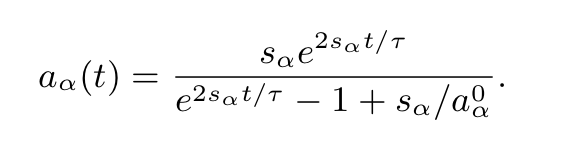
Thus, if one accepts all the assumptions we made along the way, we find that the modes of the data are learned in a stepwise manner, with the more dominant modes being learned first and faster. This is shown in the panel below:
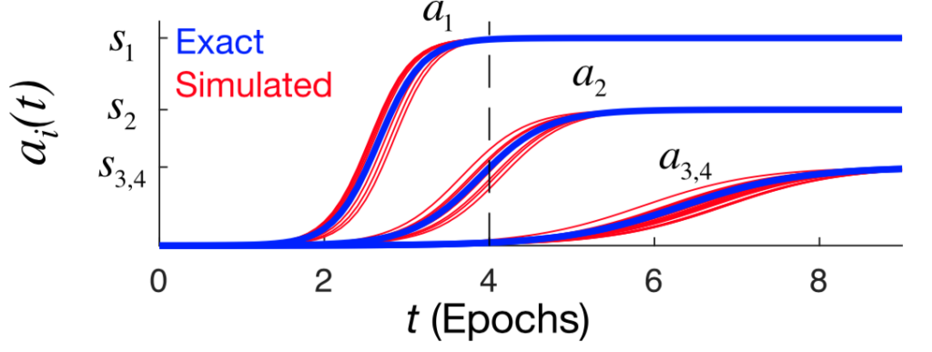
What makes a mode dominant is the number of data points it relates to. For example, the first mode is a basic “does-it-grow” mode, which all the items do. The second mode is the animal-vs-plant distinction, and so on.
Explaining the hierarchical decomposition
We can now consider how the hidden layer representations evolve over learning, to see if we can recover the phenomenon observed in the deep nonlinear networks we started this post with.
Given an input $\xx$, the corresponding representation is $$ \hh(t) = \WW_1(t) \xx = \RR \diag{\cc(t)}\VV^T \xx,$$ where $\RR$ was our arbitrary orthogonal matrix. Factoring out this term (since a fixed rotation applied to all items doesn’t change the representation), and assuming the balanced regime where $a_i(t) = c_i(t)^2$, we get $$ \hh(t) = \diag\left(\sqrt{\aa(t)}\right) \VV^T \xx.$$
Since the item representations are one-hot, $\VV^T \xx$ picks out the column of $\VV^T$ corresponding to a particular item:
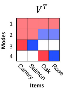
The key point is that these columns are all being premultiplied by time-varying amplitudes. For example, take the first column, corresponding to the canary, let’s call it $\cc$: $$ \cc = \VV^T \ee_1,$$ where $\ee_1 = [1,0,0,0]^T$ is the first standard basis element, and picks out the first column of $\VV^T$. When the Canary item is presented in the one-hot input $\xx = \ee_1$, the representation evolves by scaling each of the elements of $\cc$ by the time-varying amplitudes, so $$ \hh(t) = \diag\left(\sqrt{\aa(t)}\right) \cc = \begin{bmatrix}\sqrt{a_1(t)} c_1 \\ \sqrt{a_2(t)} c_2 \\ \sqrt{a_3(t)} c_3 \\ \sqrt{a_4(t)} c_4 \end{bmatrix}.$$
This scaling is done the same way for all the items, and produces a sequential activation of the elements in their representation. Early on, only the first amplitude is non-zero, so only the first row is active, and the others are zero. This means that the representation of all four items consists of the first row of $\VV^T$ above, with the remaining rows set to 0. That’s why, in the trajectory plot, all four items overlap at the beginning: their initial representations are the same.
Then, the second amplitude is acquired, adding the second row to the representation. Based on $\VV^T$ above, this now distinguishes animals and plants. Then the third activates, distinguishing the two animals from eachother, and finally the four activates, distinguishing the two plants.
Therefore, the sequential activation of the modes produces a hierarchical decomposition of representations during learning.
Conclusion
Saxe and colleagues show how two-layer linear networks learning hierarchical data learn the modes of the data sequentially, ordered by each mode’s prevalence in the data. This produces a hierarchical decomposition of representations during learning. Interestingly, this decomposition is not present in single layer networks, in which all modes are learned simultaneously and at the same rate.
Questioning the Balanced Regime
To simplify their analysis, the authors assume that that parameters are in the balanced regime, where the diagonal elements of $\overline{\WW}_1$ and $\overline{\WW}_2$, $c_\alpha$ and $d_\alpha$, are roughly the same size. James asked whether this was a valid assumption, or whether small deviations from this, like those that would occur in any real network, would get amplified and lead to pathological behaviour, like one set of weights shrinking while the other expands, etc.
To determine that, I plotted the vector field showing the dynamics of $c_\alpha$ and $d_\alpha$,\begin{align*} {d c_\alpha \over dt} &= (s_\alpha – c_\alpha d_\alpha) d_\alpha \\ {d d_\alpha \over dt} &= (s_\alpha – c_\alpha d_\alpha) c_\alpha \end{align*} for $s_\alpha = 1$:
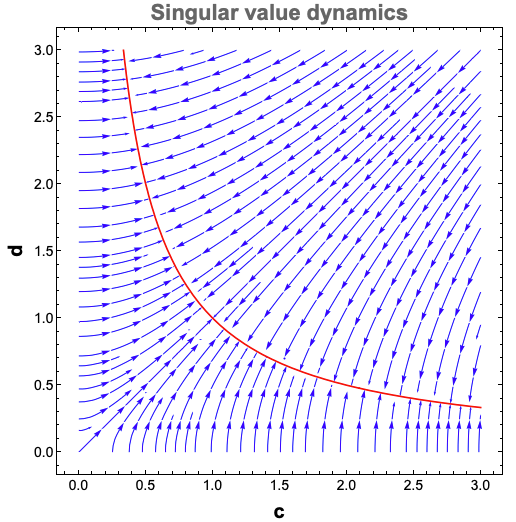
The equations tell us that the curve $c_\alpha d_\alpha = s_\alpha = 1$, drawn in red, is an equilibrium set of the dynamics. We can see above that it’s an attractor: all points converge to it. Furthermore, points the start on the diagonal remain on the diagonal. Importantly, points that start off the diagonal don’t get pushed further out. So if an initial set of points starts near the diagonal, they will stay close to it, in support of the balanced regime assumption. This effect seems amplified if the initial conditions are close to zero, as there seems to be a funnelling effect near the origin, where points get compressed towards the diagonal. Therefore, we conclude that the balanced regime is actually a good approximation of the dynamics when weights are initialized to small values.
$$ \blacksquare$$
Leave a Reply