I frequently need to differentiate loss functions with respect to matrices. I usually do this manually, which can be time-consuming and error-prone. Therefore I wanted to see if I could use Mathematica to compute these symbolic derivatives automatically. Mathematica does not have such functionality built in, but ChatGPT suggested achieving it using pattern matching.
The loss function we’ll differentiate is $$ L(R) = {1 \over 2} \|A^T (J + R)^T (J+R) A – D\|_F^2 + {\lambda \over 2}\|R\|_F^2.$$
Manual differentiation
Let’s first differentiate the loss by hand to see what the right answer is. Letting $H = A^T (J + R)^T (J+R) A – D$, we have $$ \begin{align}L(R) &= {1 \over 2} \tr(H H^T) + {\lambda \over 2}\tr(R R^T)\\
dL &= \tr(dH^T H) + \lambda \tr(dR^T R)\\
&= \tr(2 A^T dR^T (J + R)A H) + \lambda \tr(dR^T R)\\
&= \tr(2 dR^T (J + R)A H A^T ) + \lambda \tr(dR^T R)\\
&=\tr(2 dR^T (J+R)A(A^T (J + R)^T (J+R) A – D)A^T + \lambda \tr(dR^T R).
\end{align}$$ Therefore,
$$\boxed{\nabla_R L= 2 (J+R)(A A^T (J + R)^T (J+R) A A^T -A DA^T) + \lambda R.}$$
That wasn’t so bad. Let’s now try to get the same thing by applying transformation rules.
Semi-automatic differentiation
There are lots of ways to do this, below is just one, and probably not the most efficient one given that I’m a Mathematica novice.
sumOfSquares[X_] := Tr[X.Transpose[X]];
L[R_] := 1/2 sumOfSquares[Transpose[A].Transpose[J + R].(J + R).A - D1] + \[Lambda]/2 sumOfSquares[R]
First we’ll apply a symbolic differential.

Next we’ll apply a rule that commutes sums with differentials.

We want to bring the 1/2 factors out of the differentials, so we create a rule to commute differentials with scalars. The first line of the output below describes the rule, and the second line show the result of its application.

We want to do the same with the lambda at the end, so:

We’re aiming at $\tr[dR^T (\dots)]$, so next we commute the trace and the differential.

Our next aim is to turn this into the trace of a sum of differentials of dot product, e.g. $ \sum_i \tr[d(A_i B_i \dots)]$. To do this, we’re going to apply a sequence of rules. The first expresses that $(A + B)^T = A^T + B^T$.

The next distributes the dot product over sums, $A.(B+C) = A.B+ A.C$.

The next expresses $(A^T)^T = A$.

The next commutes transposing with scalar multiplication i.e. $(k A)^T = k A^T$.

Finally, the last distributes the differential over sums $d(A+B) = d(A) + dB$.

We will now apply these in the order I found by trial and error to be effective. The ‘/.’ applies the rule once, ‘//.’ applies it repeatedly until the expression doesn’t change.

The next rule distributes transpose over dot products $(A B)^T = B^T A^T$

The next rule extracts out the annoying minus signs from dot products: $A B (-C)D = -ABCD$.

Next we apply Leibniz’s rule to expand out the differentials, $d(AB) = d(A)B + A d(B)$. This produces a very long output which I’ve truncated.

Our next aim is to move all the transposed differentials to be left-most in their terms, and the un-transposed differentials to be right-most, using the circular property of the trace, $\tr(AB) = \tr(BA)$.

We next apply a transpose to end up with all terms having transposed differentials at the left-most position. We can then read off their contributions to the gradient as whatever the transposed differentials are being dot-producted against.

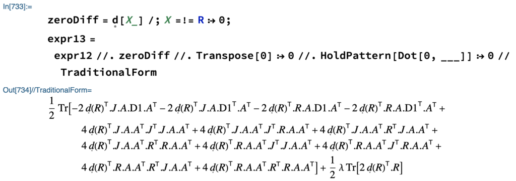
We only care about differentials of $R$, so we now zero-out the other terms.

Rather than having one big trace we distribute the trace over sums, $\tr(A+B) = \tr(A)+ \tr(B)$.

We pull out the constant terms by computing trace with scalar multiplication, $\tr(a X)$ = a \tr(X)$.

We can now extract the gradient as the sum of the terms being dot-producted against $d(R)^T$.

$D1$ is a diagonal matrix, so $D1^T = D1$.

Next we’re going to collect some dot product. First, using $AB + AC = A(B+C)$.

Next, using $BA + CA = (B+C)A$.

Next, that $k BA + k CA= k( B+ C)A$.

Next, that $ p A B + q A C = A (p B + qC)$.

Finally, we collect transposes, $A^T + B^T = (A+B)^T$.

Ideally, I’d pull out the factor of 2 as well, but couldn’t quite get that to work. Nevertheless, this is the same equation we derived manually above.
Summary
While we did get the right derivative in the end, the process was very ad hoc and even more laborious than manual differentiation. Having to hard-code the rules was interesting because it made me realise how many of these rules we apply, in problem-specific order, to arrive at the gradient. I suppose that’s part of the fun! This was an interesting exercise, but I think I’ll continue to derive my gradients manually for now.
Leave a Reply