I presented “The low-rank hypothesis of complex systems” at journal club yesterday (my post summarising it is here). During my presentation I got some interesting comments from the audience which I wanted to discuss in this post. I’ll first give the required background, then discuss the comments.

Background

In the first part of the paper, the authors provide empirical evidence that many real-world complex networks have interaction matrices with low effective rank. In the second part, they wonder whether low effective rank produces low-dimensional dynamics in such networks.

To that end, they consider the high-dimensional dynamics $$ \dot x = f(x),$$ and search for a low-dimensional linear projection of the high-dimensional space, $$x \mapsto Mx \triangleq X,$$ and a corresponding vector field in that space, $F(X)$, which matches the high-dimensional field somehow.

The “natural” way to measure the match is to compare the projection of the high-dimensional field, $M f(x)$, to the low-dimensional field, $F(Mx)$. This gives the error function $$\boxed{\veps(x;M,F) = \|M f(x) – F(Mx)\|,}$$ where we’ve made the parameterization by $M$ and $F$ explicit.

We could then sum the errors over all points in the high-dimensional space, $$\mathcal{E}(M, F) = \int_{\mathbb{R}^N} \veps(x;M,F)\; dx,$$ and minimize this function over $M$ and $F$ to arrive at a solution: a linear projection to a low-dimensional subspace, and a vector field that lives there.

The authors claim that this is difficult (more on this below), so instead take another approach and consider a different error function. Instead of projecting the high-dimensional vector field, they first project the high-dimensional input $x$ to the low dimensional space to get $M^\dagger M x$. Notice that we use the pseudo-inverse to lift the projection $Mx$ into the high-dimensional space.

They then evaluate the high-dimensonial field at the projection, and compare it to the value of the low-dimensional field at the same location. This gives the error function $$ \boxed{\mathcal{E}(x) = \| f(M^\dagger M x) – M^\dagger F(Mx)\|.}$$ Notice that we had to lift the low dimensional field with the pseudo-inverse to be able to compare it to the high-dimensional one.

The advantage of this error function over the first is that it gives an immediate solution. We solve for $F(Mx)$ by trying to set the argument in the error function to zero. Left multiplying both terms by $M$ gives the least-square solution $$F^*(Mx) = M f(M^\dagger Mx).$$ Recognizing $Mx$ as $X$, we get $$\boxed{F^*(X) = M f(M^\dagger X).}$$

Comments from the audience

I received a few interesting questions from the audience.

First comment

The first was that the second error function $\mathcal{E}(x)$ seems more restrictive than the first, $\veps(x)$. This is because in the first, we’re comparing a projection of the high-dimensional field to our low dimensional field. In the second formulation, we’re comparing the high-dimensional field in its entirety to the low-dimensional field. This seems more restrictive, since in the latter case it constrains the full high-dimensional field, not just a projection of it.

I don’t think this is actually the case. Although in the second approach we’re indeed trying to match the full high-dimensional field the low-dimensional field can only capture a projection of it. This also shows up in the solution, where $F^*(X) = M f(M^\dagger X)$. Notice that the high-dimensional field is still being projected. The difference between the two cases is where we evaluate the high-dimensional field. In the first approach, we evaluate it at an arbitrary point in the ambient space, while in the second we evaluate it on the projection of that point onto the low-dimensional subspace.

Second comment

Another comment was that the authors claim that minimizing the natural objective over both $M$ and $F$ is hard. So instead they minimize the second objective, but assuming M is known. If we assume $M$ is known, doesn’t that simplify the first minimization, perhaps yielding a solution by nonlinear regression?

Assuming that $M$ is known does simplify the first minimization, and actually yields a closed form solution, which however is hard to evaluate.

Recalling the definition of the first error function, $$ \veps(x) = \|M f(x) – F(Mx)\|,$$ we see immediately that we can set it to zero at a given point $x$ by setting $F(Mx) = M f(x).$ We want to minimize the error over the entire high-dimensional space, and since there are many points $x$ that project to same point $Mx$, least-squares tells us that the vector field at the projection is the average of the contributions from all those points. That is, $$ \boxed{F^*(X) = M \int_{Mx = X} f(x) \; dx,}$$ where we’ve dropped a constant normalizing factor.

So, even if $M$ is known, computing the integral above will probably be difficult.

Comparing the two solutions, we see that the authors’ proposed solution uses the projection of the high-dimensional field evaluated on the low-dimensional subspace, whereas the solution to the “natural” minimization is the projection of the high-dimensional field averaged over all points that project to the same point in the low-dimensional space.

When is a vector field low-dimensional?

Reflecting on the comments above made me realize that I hadn’t thought through what makes a vector field low-dimensional, nor which, if either of these notions of dimensionality reduction of vector fields, is the correct one.

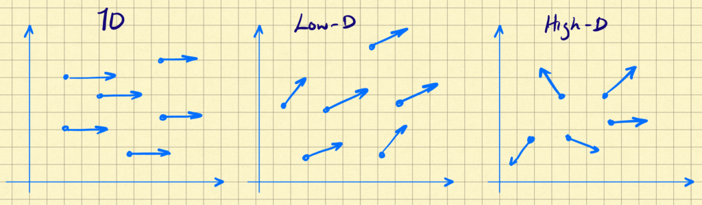
Intuitively, a vector-field is low-dimensional if the vectors all point in roughly the same direction, or within a small subspace relative to the ambient space. I show this schematically below:

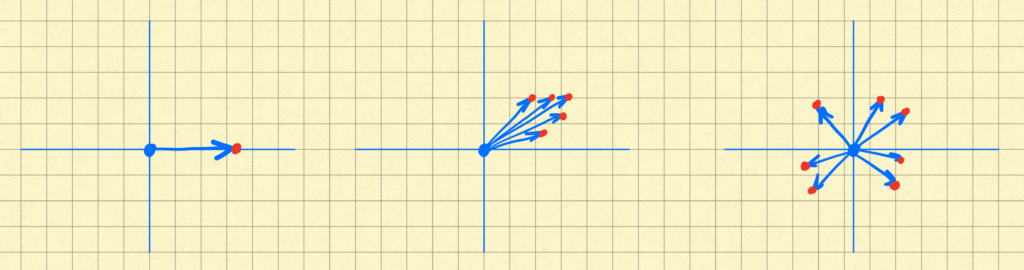
Therefore, one way we can define the dimensionality of a vector field is analogous to how we would define it for any other dataset. We select some base points at random, transport all of these along with their vectors to the origin, replacing each vector (now all originating at the origin) by the point at its terminus. We can then consider the dimensionality of the resulting point clouds. I show this schematically below for the vector fields above, with the point clouds so generated in red.

For concreteness, let’s assume we’re in $\mathbb{R}^N$, we can pick $M$ base points at random, stack the field values at those base points into the columns of an $N \times M$ matrix, which can call $f_M$. We can then compute the singular values of $f_M$, and compute dimension as usual from those. The dimension of the vector field can then be defined as the limiting value of the dimension computed in this way, so something like $$ \dim(f) \triangleq \lim_{M \to \infty} \dim(f_M).$$ A low-dimensional vector field is one for which a low-dimensional basis exists that mostly captures most vectors.

A different notion of dimensionality

By construction, the notion of dimensionality above has no notion of place – we threw away information about the base points when we transported them all to the origin, and focused on the vectors themselves.

In contrast, the notion the authors use starts with the base points $x$ in the high-D space, and looks to reduce the dimension of these to $Mx$, and find an appropriate low-dimensional vector field $F$ on the reduced space.

This is because the authors are interested in dynamics. Their notion of dimensionality reduction is not just of describing the vector fields, but of also capturing the dynamics.

One way to see how our earlier notion is not appropriate is to note that its invariant to permutation of the base points. However, such permutations would completely disrupt the dynamics.

So their notion of dimensionality reduction asks whether there is a dimension reduction of the state variables, and a corresponding induced low-dimensional dynamics, that somehow captures the high-dimensional dynamics. It’s more than just efficiently capturing the individual vectors in the vector-field.

In physics terminology, we want to find a set of low-dimensional observables and corresponding interactions whose dynamics somehow capture those of the high-dimensional system.

Which error function to use?

Given a dimension reduction of the state variables to $X = M x$, it’s natural to compare a proposed low-dimensional dynamics $F(X)$ to the dynamics induced by the projection, $\dot X = M \dot x = M f(x)$. We can measure the discrepancy using least squares error, to arrive at their initial error function, $$ \veps(x) = \|M f(x) – F(X)\|.$$

Clearly we can minimize this by setting $F(X) = M f(x)$, but we’d like the low-dimensional vector field to depend only on the low-dimensional observables.

A bigger problem with this is that it doesn’t work, conceptually. Let’s go back to the 2D vector fields above, and consider the first one. Let’s assume the vector field is a constant value of (1,0), i.e. pointing right at unit strength, everywhere. These are the blue arrows in the schematic below:

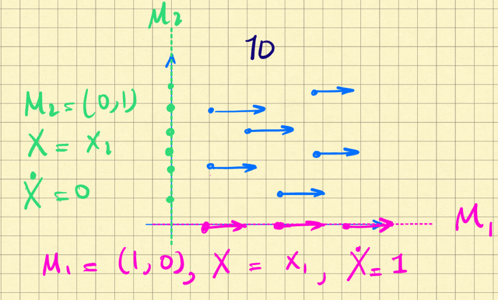
If we pick our projection to be $M_1 = [1, 0]$, then $X = x_1$. The projected dynamics are $M_1 f(x) = [1, 0]$. This is shown in pink above. The vector field $F(X) = 1$ exactly captures the projection, reduce $\veps(x)$ to zero everywhere, and describes the high-dimensional dynamics. Great.

But we can also pick the projection be $M_1 = [0,1]$. Then $X = x_2$, and projected vector field is $M f(x) = 0$ everywhere. This is shown in green above. The problem is that $F(X) = 0$ captures this projection just as well, i.e. $\veps(x) = 0$ everywhere. This despite the fact that the low-dimensional vector field doesn’t capture anything at all!

The problem is clearly that the projection of $f(x)$ can hide the deficiencies of our low-dimensional model. We should therefore compare our model to $f(x)$ itself somehow, and this is in fact what the authors resort to, but for reasons of analytic tractability. The question remains of where to evaluate $f$.

The natural place is $x$, the point in high-D, itself. So our loss becomes $$E(x) = \|f(x) – M^\dagger F(M x)\|,$$ and in fact has the same minimum we saw before, $$ F^*(X) = M \int_{Mx = X} f(x) \; dx. $$

However, we want $F(X)$ to be determined based on $X$ alone, and without assuming access to the high-dimensional variables $x$, the natural place seems to be on the low-dimensional manifold itself where $X$ lives. So, given a value of $X$, we compare the high-dimensional field at that point, $f(M^\dagger X)$, to our model of the field $M^\dagger F(X)$. Computing the error between the two gives the second error function, $$\mathcal{E}(x) = \|f(M^\dagger X) – M^\dagger F(X)\|.$$ As we showed above, this gives the low-dimensional vector field as $F^*(X) = M f(M^\dagger X)$, the low-dimensional projection of the high-dimensional field evaluated on the low-dimensional subspace.

Summary

We can summarize the discussion by stating that the error you actually should be minimizing is $E(x)$, that between the high-dimensional field $f(x)$ and its low dimensional model $M^\dagger F(Mx).$ However, the solution requires (a) evaluating a potentially complicated integral, and (b) access to the high-D state. Therefore you settle for comparing the field in the low-dimensional space to its model on that space, using $\mathcal{E}(x)$, and that gives the solution the authors arrive it. And you definitely don’t want to be comparing the projection of the high-D field to its model, using $\veps(x)$, because the projection throws away information, and can make it seem that your projection has captured the high-D field, when it has not.

$$\blacksquare$$

Appendix

Finding the Optimal Subspace

Can we use the results above to determine the optimal subspace?

The error above measures the portion of $f$ that lies outside the plane, $$\mathcal{E}(x) = \|f(M^\dagger X) – M^\dagger F(X)\| = \|f(M^\dagger X) – M^\dagger M f(M^\dagger X)\|.$$

Note first that if we were comparing $f(x)$ to its projection $M f(x)$, then the equations above, integrated over the whole space, would yield the PCA reconstruction loss, $$L_\text{PCA}(M) = \int \|f(x) – M^\dagger M f(x)\| \; dx.$$ This would be minimized when $M$ contained the top principal components of $f(x)$. That is, the solution given by our initial notion of dimensionality reduction that just focused on representing the vectors $f(x)$ efficiently.

However, we’re not using $f(x)$ but its value $f(M^\dagger x)$ on the low-D subspace. Letting $P$ be the projection $M^\dagger M$, we get $$\mathcal{E}(x) = \|f(M^\dagger X) – P f(M^\dagger X)\| = \|P_\perp f(M^\dagger X)\| = \|P_\perp f(P x)\|.$$

Since $x = P x + P_\perp x$, we can compute the error for a given $P$ as \begin{align*}\mathcal{E}(P) &= \int_x f( P x)^T P_\perp f( P x) \; dx\\ &= \int_{X = Px} \int_{X_\perp} f(X)^T P_\perp f(X) dX_\perp \; dX\\ &= \int_{X_\perp} dX_\perp \int_X f(X)^T P_\perp f(X) dX_\perp \; dX\\ &\propto \int_{X = Px} f(X)^T P_\perp f(X) \; dX .\end{align*}

This is minimized for the subspace on which the vector field has the smallest perpendicular component. But I don’t think there’s a simple closed form solution.

Error Analysis

So far, the interaction matrix relating the high-dimensional nodes hasn’t played any role in the discussion. The authors bring it in by considering computing $\veps(x)$ for their proposed $F^*(X) = M f(M^\dagger X)$. We’ve seen above that this error function is too permissive, and yet their analytical minimization of it usefully relates $W$ and $M$. Can we do the ‘correct’ analysis, using $E(x)$?

We have $$ E(x) = \|f(x) – M f(M^\dagger M x)\|.$$ We can decompose it as \begin{align*} E(x) &= \|M_\perp f(x)\| + \|M f(x) – M f(M^\dagger M x)\| = \|M_\perp f(x) \| + \veps(x).
\end{align*}

So as long as we can ensure that the components of $f$ that live off the subspace are small, their analysis goes through.