In Section 4.3.3 of his “Pattern Recognition and Machine Learning,” Bishop discusses the application of iterative reweighted least squares (IRLS) to maximum likelihood estimation of the parameters in logistic regression. The expression we get after computing the Newton-Raphson update of the parameters is $$ \ww^\text{(new)} = (\bPhi^T \RR \bPhi)^{-1} \bPhi^T \RR \zz,$$ where $$ \zz = \bPhi \ww^\text{(old)} – \RR^{-1}(\yy – \tt).$$ At the end of the section $\zz$ miraculously appears as a linear approximation to the logistic sigmoid. Is this just a coincidence?
Some questions
Bishop observes that the express for $\ww$ is the normal equation for a weighted least-squares problem, but doesn’t comment much further, leaving the following questions:
- Where does the term $\zz$ comes from?
- Why do we get a weighted-least squares problem?
- What happens if do the Newton update in terms of e.g. the drives $\aa$ to the sigmoids? How does that relate to the updates in terms of $\ww$?
- Is it just a coincidence that $\zz$ can also be derived from a linear approximation to the sigmoids?
Some answers
We’ll answer these questions below, and find that:
- We can equivalently derive the update by first computing it in the space of the drives that go into the sigmoids, $\aa$, then projecting to the parameter space $\ww$.
- $\zz$ is the Newton update to the drives $\aa$.
- Since $\aa = \bPhi \ww$, we can convert an update to $\aa$ into an update to $\ww$ by projecting into the span of the features $\bPhi$, but weighted by the curvatures of the loss relative to the drives, computed at our current estimate. Hence the weighted least-squares problem.
- The three previous points apply generally to whatever loss we’re using. Point 4 holds coincidentally for the logistic loss and logisitic activation functions. But it’s not a general property, i.e. it doesn’t hold if we swap the logisitic sigmoid out for the inverse probit.
Least Squares
To arrive at those answers, let’s start with least squares. Suppose we have $N$ independent observations $t_1$ to $t_N$, and we want to adjust corresponding output variables $a_1$ to $a_N$, to match these. We use a squared loss to measure the difference. So, packing the $\{a_n\}$ into the vector $\aa$, we have $$ E(\aa) = \sum_n {1 \over 2} (t_n – a_n)^2 = {1 \over 2} \|\tt – \aa\|_2^2.$$
The simplest possible case is when we don’t put any restrictions on $\aa$. In that setting, the solution is to set each $a_n$ to match the corresponding $t_n$: $$ \aa^* = \tt.$$
Next, let’s say that we’re no longer free to set $\aa$ arbitrarily. Instead, we have parmeterized it as living in the span of some fixed set of features. So, $$ a_n = \bphi_n^T \ww,$$ or in vector form, $$\aa = \bPhi \ww.$$ We are now looking for the $\ww$ that minimizes the loss.
Intuitively, we might guess that the optimal $\ww$ is the one that produces an $\aa$ as close as possible to the $\aa^*$ we found above. Since the $\aa$’s that we can produce are the span of $\bPhi$, we’re then looking for the orthogonal projection of $\aa^*$ onto the span of $\bPhi$. Our loss is then
$$ E(\ww) = {1 \over 2} \sum_n (t_n – \bphi_n^T \ww)^2 = {1 \over 2} \|\tt- \bPhi \ww\|_2^2.$$ If we minimize this loss we get $$\ww^* = (\bPhi^T \bPhi)^{-1} \bPhi^T \tt = (\bPhi^T \bPhi)^{-1} \bPhi^T \aa^*,$$ from which we get our estimate of $\aa$ as $$\hat \aa = \bPhi \ww^* = \bPhi (\bPhi^T \bPhi)^{-1} \bPhi^T \aa^*.$$ This is indeed the orthogonal projection of $\aa^*$ into the span of $\bPhi$, as we guessed.
Weighted Least Squares
The reason why the orthogonal projection of $\aa^*$ onto the span of $\bPhi$ was the solution is because our loss function measures deviations from the optimal value $\aa*$ along each direction equally. Minimizing the loss corresponds to adding up the squares of these deviations, which amounts to minimizing the ordinary Euclidean distance of the projection from the optimal value.
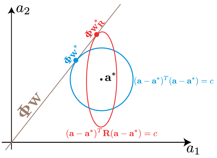
This is shown schematically for the case of two dimensions (observations) in the figure below. The span of $\bPhi$ is shown in brown. To find the least-squares projection of $\aa^*$ onto the span, we can construct balls of fixed radius around $\aa*$, and increase the radius until the ball meets the span. The corresponding ball is shown in blue below, and the intersection $\bPhi \ww^*$ with the span, marked with a blue dot.
However, we can choose to weight some samples differently. For example, we might know that some observations are noisier than others. We therefore want to weight the cleaner observations more heavily when computing our estimate. To do so, we can form a weighted loss,
$$E_R(\ww) = {1 \over 2} \sum_n r_n (t_n – \bphi_n^T \ww)^2 = {1 \over 2} (\tt – \bPhi \ww)^T \mathbf{R} (\tt – \bPhi \ww).$$
Thinking probabilisitically, our loss corresponds to the negative log likelihood of a linear Gaussian model of the observations with observation-specific precisions $r_n$: $$ p(t_n | \bphi_n) = \mathcal{N}(t_n | \bphi_n^T \ww, 1 / r_n). $$
The solution is again a projection into the span of $\bPhi$, but this times a weighted projection, favouring the cleaner observations. To find it, we set the gradient of the loss to zero and get \begin{align*} 0 &= \sum_n r_n (t_n – \bphi_n^T \ww) \bphi_n = \bPhi^T \RR \tt – \bPhi^T \RR \bPhi \ww\\ \implies \ww^*_\mathbf{R} &= (\bPhi^T \RR \bPhi)^{-1} \bPhi^T \RR \tt = (\bPhi^T \RR \bPhi)^{-1} \bPhi^T \RR \aa^*,\end{align*} from which our weighted least-squares projection becomes $$\hat \aa_\mathbf{R} = \bPhi \ww^*_\mathbf{R} = \bPhi (\bPhi^T \RR \bPhi)^{-1} \bPhi^T \RR \aa^*.$$
We can find this solution by starting at $\aa^*$ and expanding out balls of fixed weighted radius. This is shown schematically in red in the figure above. The balls of fixed weighted radius are elliptical, with axis lengths corresponding to the standard deviations of the noise in the probabilistic interpretation, $1/\sqrt{r_n}$. In the schematic above, the first observation $a_1$ has a larger weight, corresponding to a smaller standard deviation, than the second observation. This results in the projection, $\bPhi\ww_R^*$ being closer to $a_1^*$ than $a_2^*$.
Newton-Raphson updates
Often our loss function is more complicated than the squared loss we’ve been using above, so that even with full control of our outputs, $\aa$, it might not be clear what value to set them to to minimize the loss. If we have gradient information, we can certainly try reducing the loss by gradient descent. However, if the loss function is well-behaved, we can sometimes get faster convergence by also using curvature information.
To do so, we can assume that our loss function is quadratic, with curvature given by whatever it is at our current location, which we call $\aa_t$. To update our location to $\aa_{t+1}$, we assume assume that $$E(\aa) \approx {1 \over 2} (\aa – \aa_{t+1})^T \RR_t (\aa – \aa_{t+1}),$$ where $\RR_t = \nabla_\aa^2 E$ is the Hessian of the loss at $\aa_t$, the matrix of second derivatives with respect to the elements of $\aa$. The value $\aa_{t+1}$ is the value of $\aa$ that will minimize this quadratic approximation of the loss. Notice that we again have a weighted least squares problem.
To find $\aa_{t+1}$, we consider changing our output $\aa$ by some amount $\Delta$. This would change the gradient to$$ \nabla_\aa E(\aa + \Delta) \approx \nabla_{\aa} E + \nabla^2_{\aa} E \Delta.$$ At the optimum the gradient of our loss should be zero. Therefore, we can find the update by setting the expression to zero and solving for $\Delta$, to get $$ \Delta_\aa = – (\nabla_{\aa}^2 E)^{-1} \nabla_{\aa} E.$$ This gives the Newton-Raphson update of our outputs as
$$ \aa_{t+1} = \aa_t – (\nabla_{\aa}^2 E)^{-1} \nabla_{\aa} E.$$
Newton-Raphson as weighted least squares
What if we don’t control the outputs $\aa$ themselves entirely, but only a subspace $\bPhi \ww$? We can perform a Newton-Raphson update of $\ww$. How is this update related to that of $\aa$? We can find the update in two ways.
The easy way is to return to our quadratic approximation of the loss and express it in terms of $\ww$ instead of $\aa$: $$E(\aa(\ww)) = {1 \over 2}(\aa_{t+1} – \bPhi \ww)^T \RR_t (\aa_{t+1} – \bPhi \ww).$$
But this is just a weighted least-squares problem, whose solution we already found above to be
$$\ww_{t+1} = (\bPhi^T \RR_t \bPhi)^{-1} \bPhi^T \RR_t \aa_{t+1}.$$
We can verify that is indeed the Newton-Raphson update of $\ww$ by computing it directly. We have $$ dE(\aa(\ww)) = \nabla_\aa E^T d\aa = \nabla_\aa E^T \bPhi d\ww \implies \nabla_\ww E = \bPhi^T \nabla_\aa E.$$
Then $$ d\nabla_\ww E = \bPhi ^T d\nabla_a E = \bPhi^T \nabla_a^2 E d\aa = \bPhi^T \nabla_\aa^2 \bPhi d\ww,$$ from which we get $$ \nabla_\ww^2 E = \bPhi^T \nabla_\aa^2 \bPhi.$$
Combining the pieces, we get the Newton-Raphson update of $\ww$ as
\begin{align*} \Delta_\ww &= -(\bPhi^T \nabla_\aa^2 \bPhi)^{-1}\bPhi^T \nabla_\aa E\\&= (\bPhi^T \nabla_\aa^2 \bPhi)^{-1}\bPhi^T \nabla_\aa^2 (-(\nabla_\aa^2 E)^{-1}\nabla_\aa E) \\ &= (\bPhi^T \RR_t \bPhi)^{-1}\bPhi^T \RR_t \Delta_\aa,\end{align*} where $\RR_t$ is the curvature $\nabla_\aa^2 E$ at the current value of $\aa$. This says that the change to $\ww$ is the weighted least-squares projection of the change to $\aa$.
To get the the updated value of $\ww$ we expand the $\Delta$’s, \begin{align*} \ww_{t+1} &= \ww_t + \Delta_\ww\\ &= \ww_t + (\bPhi^T \RR_t \bPhi)^{-1}\bPhi^T \RR_t (\aa_{t+1} – \aa_t)\\&= \ww_t + (\bPhi^T \RR_t \bPhi)^{-1}\bPhi^T \RR_t (\aa_{t+1} – \bPhi \ww_t)\\&= (\bPhi^T \RR_t \bPhi)^{-1}\bPhi^T \RR_t \aa_{t+1},\end{align*} which is the expression we derived previously.
So, we conclude that when the outputs are parameterized as $\bPhi \ww$, the Newton-Raphson update to the parameters $\ww$ is the least squares projection of the update to $\aa$, weighted by the curvature of the loss function.
Application to Logistic Regression
It turns out that the Newton-Raphson updates for the cross-entropy loss of logistic regression have a particularly simple form.
The loss is $$E(\aa) = -\sum_n t_n \log \sigma(a_n) + (1 – t_n) \log (1 – \sigma(a_n)).$$
Writing $\sigma(a_n)$ as $\sigma_n$, the gradient is $$ {\partial E \over \partial a_n} = \left(- {t_n \over \sigma_n} + { 1 – t_n \over 1 – \sigma_n}\right) {d\sigma_n \over da_n} = \left(\sigma_n – t_n \over \sigma_n (1 – \sigma_n) \right) {d\sigma_n \over da_n} .$$
Now it just so happens that for the logistic sigmoid, $d\sigma_n/da_n$ equals the denominator in the expression above. Therefore, the gradient simplifies to $${\partial E \over \partial a_n} = (\sigma_n – t_n).$$
The curvature is simple to derive from this as $$ r_n \triangleq {\partial^2 E \over \partial a_n^2} = {d \sigma_n \over d a_n} = \sigma_n (1 – \sigma_n).$$
The Newton-Raphson updates of $\aa$ are now simply $$ a_n^\text{(new)} = a_n^\text{(old)} + {t_n – \sigma_n \over \sigma_n (1 – \sigma_n)}.$$ Packing the curvatures $r_n$ into the diagonal matrix $\RR$, we can write this in vector form as $$\aa^\text{(new)} = \aa^\text{(old)} + \RR^{-1} (\tt – \sigma(\aa)).$$
Performing a weighted least squares projection of this updates into the span $\bPhi$ gives the update to the parameters, \begin{align*}\ww^\text{(new)} &= (\bPhi^T \RR_t \bPhi)^{-1}\bPhi^T \RR_t(\bPhi \ww^\text{(old)} + \RR_t^{-1} (\tt – \sigma(\aa))\\&= \ww^\text{(old)} + (\bPhi^T \RR_t \bPhi)^{-1}\bPhi^T \RR_t \RR_t^{-1} (\tt – \sigma(\aa))\\&= \ww^\text{(old)} + (\bPhi^T \RR_t \bPhi)^{-1}\bPhi^T (\tt – \sigma(\aa)).\end{align*} where we’ve replaced $\aa^\text{(old)}$ with $\bPhi \ww^\text{(old)}.$
A spurious coincidence
Instead of Newton updates, we can consider having taken another approach. Our outputs are logistic functions $\sigma(a_n)$ of inputs $a_n = \bphi_n^T \ww.$ We can consider performing a first-order update of $\sigma$ to match $t_n$: $$t_n = \sigma(a_n + \delta a_n) \approx \sigma(a_n) + {d\sigma \over da_n}\delta a_n.$$ From this we get $$\delta a_n = \left({d\sigma \over da_n} \right)^{-1} (t_n – y_n) = {da_n \over d\sigma} (t_n – y_n)= r_n^{-1}(t_n – y_n).$$ This culminates in $$ a_n^\text{(new)} = \bphi_n^T \ww^\text{(old)} + r_n^{-1}(t_n – y_n) = z_n.$$
In other words, our first order update to $\aa$ provides the target that’s used in the WLS update to $\ww$, which is a second order update in $\ww$. Is this is a coincidence?
The Newton update to $\aa$ is $$ \Delta_\aa = -(\nabla_\aa^2 E)^{-1} \nabla_\aa E.$$ We can assume that our loss will be minimized if we make the output activations equal the observations, that is if we set $\sigma(a_n)$ to match $t_n$. A linear approximation like the one above is then a reasonable idea. But this will not correspond to the Newton update in general (i.e. for activations other than the logistic sigmoid).
For example, if use the logistic loss but replace $\sigma(a)$ with inverse probits, $$ f(a) = {1 \over 2}\left(1 + \text{erf}\left({a \over \sqrt{2}} \right)\right),$$ we have $$f'(a) ={1 \over \sqrt{2\pi}}e^{-a^2/2}.$$ Then
$$ \nabla_a E = {f – t \over f (1 – f)} f'(a),$$ but we no longer get the cancellation between the denominator and the $f'(a)$. The curvature is
$$ \nabla_a^2 E = {f’^2 \over f(1 – f)} – {f -t \over f^2(1-f)^2}(1 – 2f)f’^2 + {f – t \over f(1 -f)} f’\hspace{0cm}’.$$ Combining this with the gradient to get the Newton update is not going to yield a simple linear expression in $(t – f).$
So yes, for the logistic loss using the logistic sigmoid, one can think of $\zz$ as being derived from the linear approximation above. But this only applies for this particular combination of loss and activation function, and the relationship doesn’t hold in general.
The better way to think about $\zz$, which does hold in general, is as the Newton update to $\aa$. Its form will change depending on the loss and the activation, but conceptually, that’s what it is, and a weighted projection of it gives the update to the parameters $\ww$.
$$\blacksquare$$
Leave a Reply