These notes are based on Seung’s “How the Brain Keeps the Eyes Still”, where he discusses how a line attractor network may implement a memory of the desired fixation angle that ultimately drives the muscles in the eye.
A Jupyter notebook with related code showing how to implement a line attractor is provided here.
Background
Why keep the eyes still?
The brain needs to keep the eyes still to allow the visual system to process the image on the retina. Nystagmus is a medical condition where patients’ eyes exhibit involuntary movement. This lack of fixation can mean that their vision is impaired, even though all the other machinery in the visual system is working correctly. The clip below shows an example of a patient with nystagmus.
The relevant anatomy
To keep things simple, Seung focuses on the horizontal movement of the eye. The relevant anatomy is shown below in a figure from “Principles of Neural Science”, 5th Edition.
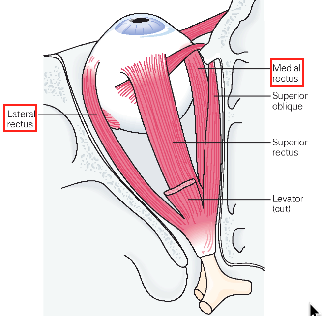
The muscles we’ll be focusing on are the lateral and medial rectus, highlighted above, which move the eye away from, and towards, the nose, respectively.
The circuit that drives these muscles is shown in another figure from Kandel, below:
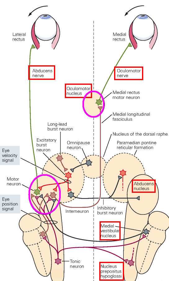
The most relevant facts for this paper are:
- The lateral rectus is driven by the abducens nerve emanating from the abducens nucleus.
- The medial rectus is driven by the oculomotor nerve, emanating from the oculomotor nucleus, which is also driven by the abducens nucleus.
- The abducens nucleus receives input from the medial vestibular nucleus (MVN) and the nucleus prepositus hypoglossi (PH).
- There are few feedback connections from the abducens and oculomotor nuclei to the MVN or PH.
- The MVN and PH contain intranuclear and bilateral feedback loops.
The relevant physiology
Some of the evidence Seung cites to suggest the various roles of the components of this system are:
- When the eyes are still, the firing rates in the abducens nucleus and oculomotor nucleus are approximately linear in eye position.
- Electrical perturbation of these areas causes a transient change in eye position, which then returns to its original position.
- Damaging the connections from the abducens nucleus to the oculomotor nucleus weakens (control?) of the medial rectus, but the eyes can still be kept still.
- Perturbation of the MVN or PH leads to lasting changes in eye position.
- Lesioning or pharmacologically inactivating these areas leads to nystagmus
- As mentioned above, the MVN and PH areas contain feedback connections both within nuclei and bilaterally.
How the Brain Keeps the Eyes Still
The abducens and oculomotor nuclei form a point attractor
Based on points 1-3 above, Seung suggests that the abducens and oculomotor nuclei form a readout of eye position. This can be implemented by a point attractor, as schematized in the figure below from Seung’s paper:
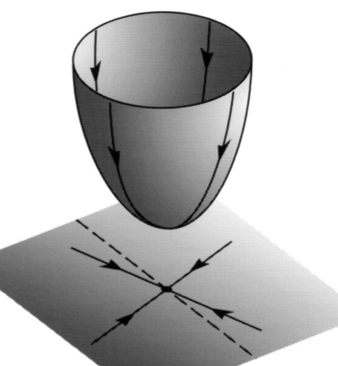
The point attractor converges to the representation of eye position provided by upstream areas. Its dynamics ensure that it is robust to perturbations.
The MVN and PH implement a memory of eye position using a line attractor
Based on points 3-6 above, Seung suggests that the MVN and PH implement a memory of eye position, and implement this through a line attractor, schematized below:
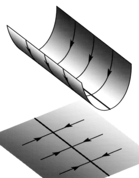
In this view, upstream areas provide the desired eye position to this memory system. Its neutral stability along its attractor dimension means that such inputs can shift its representation to the desired target state, and that representation will persist after the control input is removed. The MVN and PH communicate the desired position to the point attractor in the abducens and oculomotor nuclei.
Building a Line Attractor
In this section, we’ll show how to build a line attractor that can keep a memory of eye position. Relevant code is provided in the Jupyter notebook.
Modelling Horizontal Motion of the Eye
We begin with a simple model of the eye as a sphere mounted on a swivel, with two handles on the left and right, actuated by muscles applying a force of $F_L$ and $F_R$, respectively. The passive springiness of the eye is captured by two springs situated at the same location as the muscles, with spring constants $k$. The eye’s position is registered by the angle $\theta$ moving counter-clockwise from the neutral position. This is schematized below:
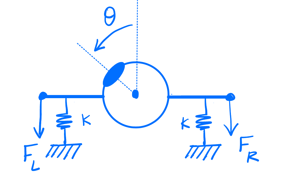
Applying different amounts of force on the two sides will rotate the eye until torque balance is achieved. Normalising units so that the muscles and springs are situated a unit length from the centre of the eye, torque balance gives us $$ F_L – k \theta = F_R + k \theta,$$ from which we get $$ \theta = {F_L – F_R \over 2 k}.$$
Drive by neurons
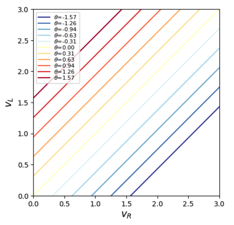
Let’s assume each muscle is linearly driven by a motor neuron, so that $v_L= F_L/2k$, and similarly for $v_R$. Then gaze position is determined by the difference of these voltages, $$ \theta = v_L – v_R.$$ The plot below shows voltages that achieve angles from $-\pi/2$ to $\pi/2$:
Controlling the Range of Motion
To drive the eye to a desired angle, we can, in principle, choose any point on the corresponding line. Connecting these gives us the control path the brain would use to drive the eyes.
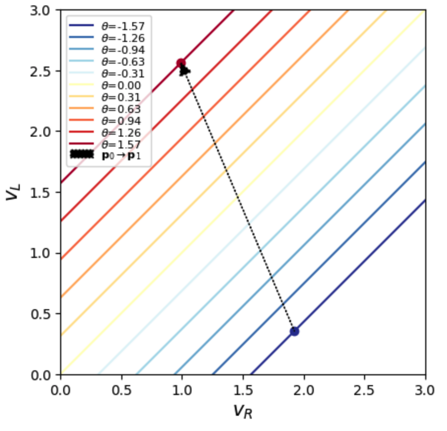
However, it seems likely that such a path would at least be continuous, to keep the brain from having to change voltages abruptly as it moves from one angle to another nearby value. In fact, it turns out that the voltages are related linearly to the desired angle, according to $$v_i = v_i^0 + k_i \theta.$$ This corresponds to a linear path through the solution space, whose slope and offset are determined by $v_i^0$ and $k_i$, respectively.
One example linear path through the solutions is shown below:
Line attractors in a 1D linear system
Let’s assume an upstream area provides the target eye direction $\theta$. How are we going to achieve the appropriate voltages for it?
One possibility would be to constantly drive the output neurons with the desired voltage. We could do this with point attractor dynamics. In a one-dimensional case, we could start with $$ \tau \dot v = -v.$$ This system has a single attractor, at $v = 0$. Adding a drive $v^*$, so $\tau \dot v = -v + v^*$, shifts this attractor to $v = v^*$, and provides the necessary input to the muscles.
The point attractor solution requires maintaining a constant drive to to the neuron to counteract its leak. Another solution would be to have the neuron remember its previous voltage. What makes it forget is its leak. Therefore, the neuron can use self-excitation to exactly counteract the leak. This makes the neuron neutrally stable, so it maintains its voltage: $$ \tau \dot v = -v + v = 0.$$ Initialised from any point on the $v$-axis, the voltage will stay there. Therefore, every point on the $v$-axis is an attractor, and we have just created our first line attractor.
How would we control this system? Since it doesn’t leak, it has perfect memory, and its output integrates its entire history. If we provide it with a drive, $u(t)$, so its dynamics are $$ \tau \dot v = u(t),$$ then it’s output at any time $T$ is $$ v(T) = \int_0^T u(t) dt.$$
To keep things simple, we can assume we drive it with impulses at times $t_i$, with amplitude $A_i$, so the drive is $$u(t) = A_1 \delta(t-t_1) + A_2 \delta(t-t_2), \dots.$$ In that case, the neuron’s voltage just sums the amplitudes of the impulses up to time $T$: $$v(T) = \sum_{t_i < T} A_i.$$
If we call its voltage before the last impulse $v(T’)$, then we see that the impulse updates the voltage: $$ v(T) = v(T’) + A_i.$$ By keeping track of the previous voltage, we can use the impulse to get the output to be whatever we want.
Line attractors in a 2D Linear System
Having built a line attractor in 1D, we’ll now build one in 2D, to control our two voltages. We’ll pack our two voltage $v_L$ and $v_R$ into the vector $$\vv = \begin{bmatrix} v_L \\ v_R \end{bmatrix}.$$
We’re still dealing with a linear system, so we’ll start with the dynamics $$ \tau \dot \vv = -\vv + \WW \vv + \ff.$$
Here $\WW$ is the matrix of synaptic weights connecting the neurons to each other. We’ve also added the background inputs $\ff$ to represent the contributions from other systems e.g. head-direction, vestibular, which we’ll take to be constant.
We now have two tasks. First, we need to determine which weights $\WW$ and background inputs $\ff$ will give us the line attractor we need. Second, we need to determine how to drive our system along this attractor to get the outputs we need.
Building the line attractor
To build the line attractor, we need the fixed points of the system to form a line. Setting $\dot \vv$ to 0, we see those fixed points satisfy $$\vv = \WW \vv + \ff.$$ In general, this system will have exactly one solution, so will operate as a point attractor. However, for special, finely tuned, values of $\WW$ and $\ff$, its solutions will lie along a line.
To find these special values of $\WW$ and $\ff$, it’s helpful to switch coordinates to the eigenvectors $\qq_1$ and $\qq_2$ of $\WW$. We can express vectors in those coordinates as, e.g. $$\vv = \qq_1 \tilde v_1 + \qq_2 \tilde v_2.$$ We can then study the dynamics in the new coordinates, $$\tau \dot{\tilde \vv} = -\tilde \vv + \widetilde \WW \tilde \vv + \tilde \ff.$$
The advantage of doing so is that the weight matrix in the new coordinates is diagonal, $$\widetilde \WW = \begin{bmatrix} \lambda_1, 0 \\ 0, \lambda_2 \end{bmatrix},$$ where $\lambda_1$ and $\lambda_2$ are the two eigenvalues. That is, rather than working with a coupled 2D system, we can deal with two uncoupled 1D systems, $$\begin{align*} \tau \dot{\tilde v_1 }&= -\tilde v_1 + \lambda_1 \tilde v_1 + \tilde f_1,\\\tau \dot{\tilde v_2 }&= -\tilde v_2 + \lambda_2 \tilde v_2 + \tilde f_2.\end{align*}$$
We’ve already dealt with 1D line attractors above! Let’s suppose we want the line attractor along the first eigen vector. We then have to make the corresponding dynamics neutrally stable. That is, we need $$ 0 =\tau \dot{\tilde v_1 } = -\tilde v_1 + \lambda_1 \tilde v_1 + \tilde f_1.$$
To achieve this, we need two conditions:
- $\lambda_1 = 1$: This corresponds to self-excitation to cancel the leak.
- $\tilde f_1 = 0$: This means the background drive must be orthogonal to the first “left” eigenvector, which in turn means it must lie along the second eigenvector. This is because any non-zero constant inputs along its attractor dimension would be integrated to infinity!
The dynamics along the other direction must be a point attractor, otherwise we’d have a plane attractor! Their fixed point is where $$ 0 =\tau \dot{\tilde v_2 } = -\tilde v_2 + \lambda_2 \tilde v_2 + \tilde f_2,$$ which gives $$ \tilde v_2(\infty) = {\tilde f_2 \over 1 – \lambda_2}.$$
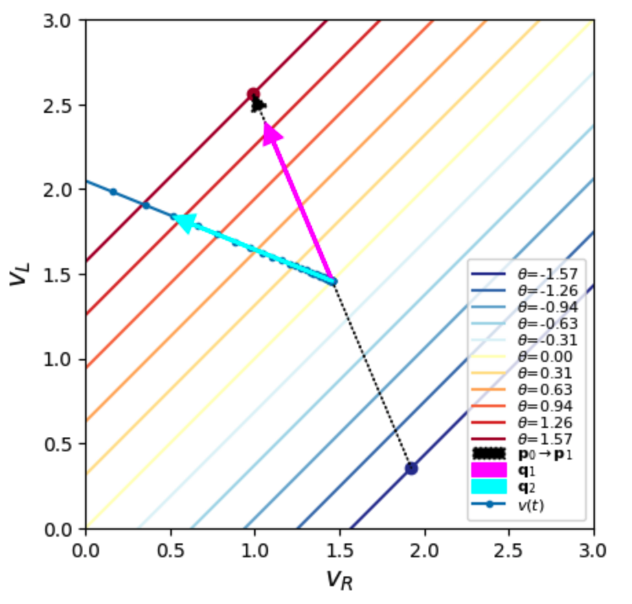
We now have a full description of our attractor: we know that it consists of a line attractor along the first eigenvector $\qq_1$, and a point attractor along the second eigenvector $\qq_2$. Combining these pieces, we can describe the voltages along our attractor as the set of points $$ \vv (\alpha) = \alpha \qq_1 + \tilde v_2(\infty) \qq_2 = \alpha \qq_1 + \overline \vv.$$ Different values of $\alpha$ correspond to different initial conditions.
Aligning the line attractor
The equation for our attractor above defines a line in the direction $\qq_1$ that passes through $\overline \vv.$ We want to set its parameters to pass through the voltage combinations we need to drive the eye. This voltage path is a line that goes from $\pp_0$ to $\pp_1$. Therefore, we know that the direction of our line must be the same, so we’ll set $\qq_1$ to be the corresponding unit vector: $$ \qq_1 = {\pp_1 – \pp_0 \over \|\pp_1 – \pp_0\|} = \hat \pp.$$
To specify the rest of $\WW$, we can set $\qq_2$, the second eigenvector, to be a different but otherwise arbitrary unit vector. We also set the second eigenvalue $\lambda_2$ to some value less than 1, ideally much less than one so that convergence to the line attractor is quick.
We’re not quite done: we need our network’s line attractor to line up with the one we’ve chosen to drive the muscles. This desired line is along the set $\pp_0 + \alpha \hat \pp.$ The line attractor for our network is along the set $\overline{\vv} + \alpha \hat \pp$. To align these, we need to shift our attractor so that its $\qq_2$ coordinates line up with those of our desired attractor.
To do so we, express $\pp_0$ in the eigenvector coordinates as $$\pp_0 = \tilde{p}_{01} \hat \pp + \tilde{p}_{02} \qq_2.$$ Our desired line attractor is then, equivalently, the set $(\alpha, \tilde{p}_{02})$ in eigenvector coordinates. Our network’s line attractor is along the set $( \alpha, \tilde v_2(\infty))$ in eigenvector coordinates. To line these we up, we simply match their second coordinates:
$$ \tilde{p}_{02} = \tilde v_2(\infty) = {\tilde f_2 \over 1 – \lambda_2},$$ which determines the $\qq_2$ coordinate of the background drive we need as $$\tilde f_2 = ( 1- \lambda_2) \tilde{p}_{02}.$$
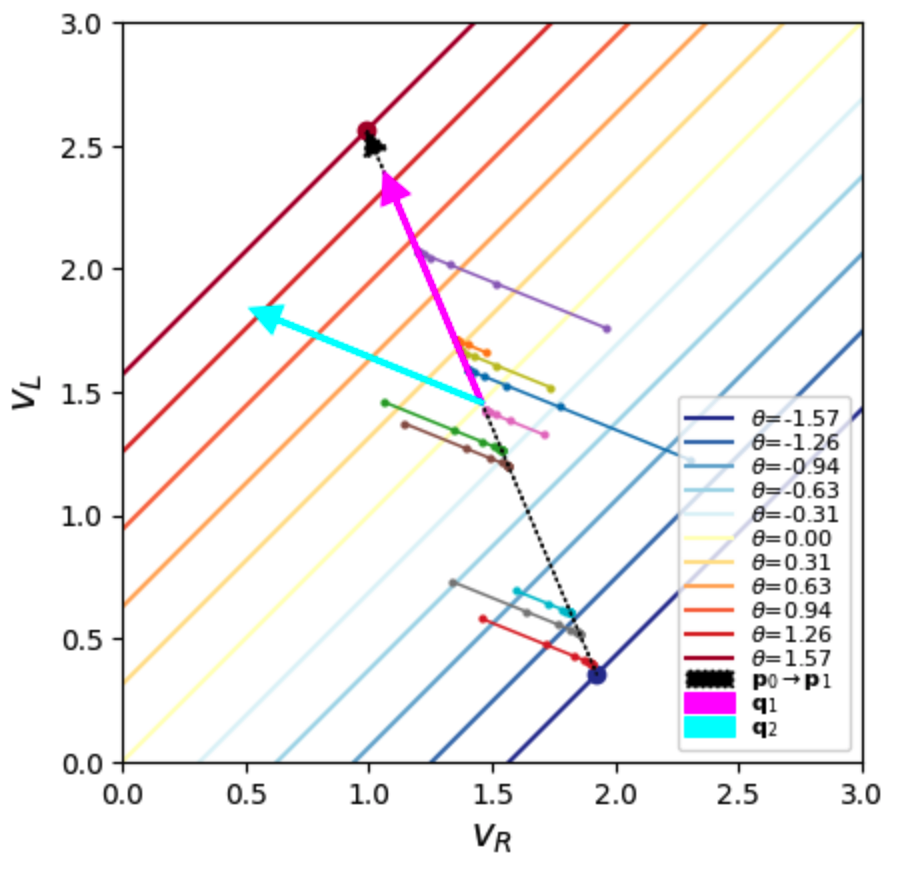
To verify that our line attractor looks the way we want, we can see where a few initial points end up. Doing so below reveals that they end up on our desired line.
Initialization
Before we introduce a control input to change the eye position, let’s first determine the initial condition we should apply to have the system settle down to the voltages corresponding to some desired initial angle $\theta_0$.
Since our voltages drive head directions linearly from $-\pi/2$ at $\pp_0$ to $\pi/2$ at $\pp_1$, the voltage pair this will correspond to is \begin{align}\vv_0 &= \pp_0 + (\pp_1 – \pp_0) {\theta_0 – (- \pi/2 ) \over \pi/2 – (-\pi/2)}\\ &=\pp_0 + (\pp_1 – \pp_0) {\theta_0 + \pi/2 \over \pi}\\ &=\pp_0 + \hat \pp \|\pp_1 – \pp_0\| {\theta_0 + \pi/2 \over \pi}.\end{align}
By design, all such points will have the same $\qq_2$ coordinates as the points along our network’s attractor, so we don’t have to worry about that coordinate. The only one we’ll need to determine is the one along $\hat \pp$. We’ll give it a tilde to indicate it’s the coordinate, and the subscript 1 to indicate it’s the first coordinate. So we get $$\tilde v_{01} = \tilde{p}_{01} + \|\pp_1 – \pp_0\| {\theta_0 + \pi/2 \over \pi}.$$ Below we show an example for $\theta_0 = 0$.
Driving the attractor
Now suppose our attractor is sitting at a position corresponding to $\theta_0$. How do we nudge it to a new desired angle, $\theta_1$?
By subtracting the coordinates $\tilde v_{01}$ we need for different values of $\theta$, we can see that the change we need is $$\Delta {\tilde v_1} = \|\pp_1 – \pp_0\| {\theta_1 – \theta_0 \over \pi} = \|\pp_1 – \pp_0\| {\Delta \theta \over \pi}.$$
This makes intuitive sense: to change the angle by some amount $\Delta \theta$, we need to change the attractor location by some proportional amount.
To provide such changes, we’ll update the dynamics along the attractor direction to receive a drive $u(t)$: $$ \tau \dot {\tilde v_1} = \tilde u(t).$$ This means, as we discussed before, that $$ \tilde v_1(T) = \tilde v_1(0) + {1 \over \tau} \int_0^T \tilde u (t) dt.$$ Therefore, $$\Delta \tilde v_1 = {1 \over \tau} \int_0^T \tilde u(t) dt.$$
If at some point $t’$ in that interval we provide an impulse of amplitude $\tau A$, so $$u(t) = \tau A \delta(t – t’),$$ then $$\Delta \tilde v_1 = {1 \over \tau} \int_0^T \tau A \delta(t – t’) dt = A.$$
Therefore, to change the angle by some amount $\Delta \theta$, we provide a drive of $$\uu(t) = \hat \pp \tilde u(t) = \hat \pp \tau \|\pp_1 – \pp_0\| {\Delta \theta \over \pi} \delta(t – t’) = \tau {\Delta \theta \over \pi}\delta(t-t’) \pp .$$
This is the intuitive result that to shift the angle by $\Delta \theta$, you nudge the system along the attractor by an amount proportional to it.
Caveats
Seung mentions several caveats of the line attractor solution.
The first caveat is that it is structurally unstable. Recall that when we were constructing our line attractor, we had to engineer our synapses so that one of the eigenvalues was exactly 1 to achieve neutral stability. Physically, this was to ensure the feedback exactly cancelled the leak. In reality, such hard-coded fine-tuning is implausible. Any biological implementation will deviate from the ideal of neutral stability and may exhibit fixed points. Some possible deviations from the line attractor are shown in Seung’s schematic below:
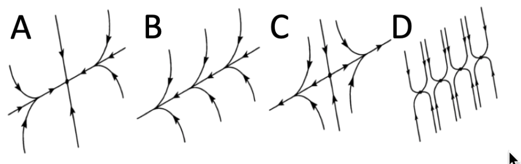
In the first, a fixed point is introduced, resulting in drift to a neutral position. In the second, no fixed points exist, producing drift in one direction. In the third, there’s a saddle point, producing a drift away from the centre. The last example shows a nonlinear system that now exhibits multiple fixed points, which would produce drift to the nearest one.
Another important caveat is that we’ve used linear systems throughout. Nonlinear systems in general will not exhibit line attractors, because there typically won’t be linear solutions to fixed-point equations of nonlinear systems. One exception is when the nonlinearity, $g$ is in the firing rate functions of the neurons. In that case, the driving voltages of the neurons at steady state according to $$\uu = \mathbf{A} g(\uu) + \hh.$$ If we engineer $\mathbf{A}$ to have be rank-1, then the solutions will always lie along a single linear direction. Seung refers a discussion of this solution to another paper.
Summary
In summary Seung shows how the evidence suggests that the important operation of keeping the eyes still may be implemented by storing the desired eye location in a line attractor network, and reading it out in a point-attractor network. Based on Seung’s approach, we showed in detail how such a line attractor network can be constructed to control the position of the eye.
$$\blacksquare$$
Leave a Reply