Recently, William Walker and colleagues proposed the Recognition Parameterized Model (RPM) to perform unsupervised learning of the causes behind observations, but without the need to reconstruct those observations. This post summarizes my (incomplete) understanding of the model.
One popular approach to unsupervised learning is autoencoding, where we learn a low-dimensional representation of our data that can reproduce it. Perhaps the simplest autoencoder is PCA, in which we try to find orthonormal projections of the data that best capture it in a least-squares sense.

Reconstructing the data makes sense in a data-analysis setting where our aim actually is capturing the full high-dimensional complexity of a dataset with appropriately chosen low-dimensional variables and projections.
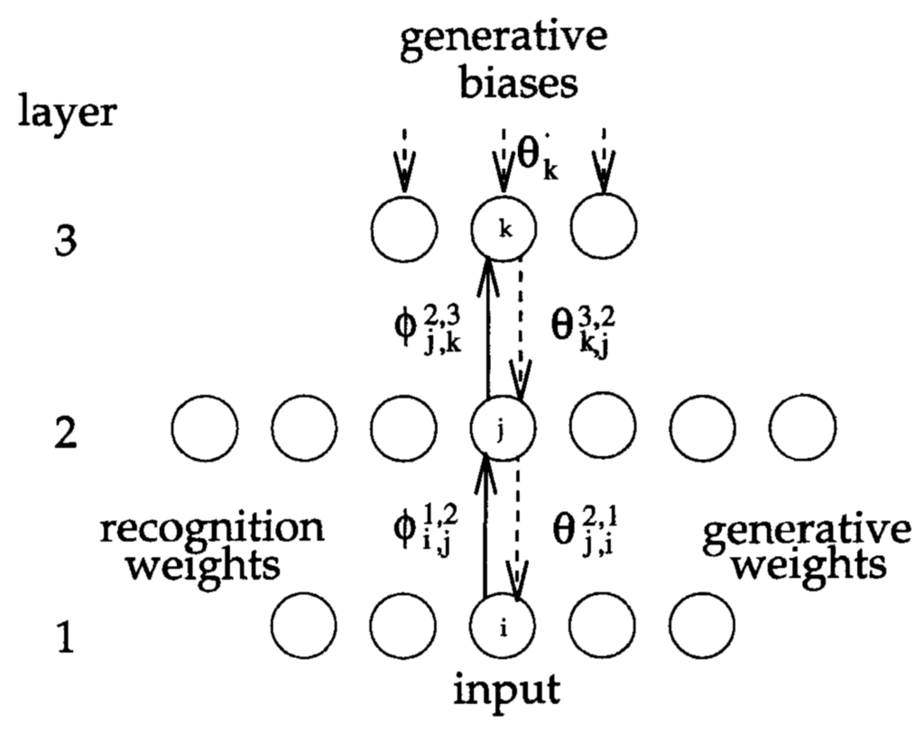
Reconstruction is also used in an influential probabilistic model of perception called the Helmholtz Machine. Inspired by Helmholtz’s notion that perception is the inference of causes from observations, the Helmholtz machine contains a recognition model that maps sensory observations to the activations of units representing causes. The parameters of this model are learned using a separate generative model that maps causes to observations. During the ‘sleep’ phase of training, the model generates causes at the deepest level of its neural network, which then percolate outwards until they ultimately produce a set of sensory inputs (‘dreams’, perhaps). The parameters of the recognition network are adjusted so that the causes it infers for these dreams match the actual causes used to generate them.

Does such reconstruction occur in the brain? Models like the Helmholtz machine require feedforward connections from the sensory stages all the way through the causal hierarchy, and feedback connections all the way back down. Although there are no feedback connections from the cortex to the retina, there is extensive feedback to at least the earliest visual layers in the cortex. So it is possible that these feedback connections are being used to reconstruct V1 activation levels. And we certainly have the experience of our dreams, in which apparently random visual stimuli are produced at what often seems to be high fidelity.
Despite these anatomical plausibilities, reconstruction seems unlikely as something that goes on in the brain for several reasons. First, the animal is not interested in reconstruction per se, but only in so far as it provides useful latents for navigating the world. Second, reconstruction means reconstruction of everything. A visual scene would have to be reconstructed in all of its detail, despite often only very small subsets of it being important to the behaviour or understanding of the animal. Third, generative models needed to reconstruct natural scenes would presumably be complex, and mismatches in these can cause biases in recognition.
The motivating question then presents itself: is it possible to do unsupervised learning of the causes underlying sensory inputs, without reconstructing those inputs? That is, using a recognition model, but no generative model?
The answer is: Yes! Instead of using a generative model to train its recognition model, the RPM uses the assumed conditional independence of observations given the latents. That is, it doesn’t search for latents that can then be plugged into a generative model to reconstruct sensory observations. Rather, it looks for latents that make those observations conditionally independent.
By avoiding using observation reconstruction to train the recognition model, the RPM (a) avoids generative model mismatch issues since none is being used, and (b) avoids expending computational resources capturing irrelevant components of the sensory input.
The Recognition-Parameterized Model
To derive the RPM, we assume that we observe the values of $J$ sensory inputs, $X = \{\xx_1, \dots, \xx_J\}$. These $J$ inputs can be vector-valued. For example, they can represent the pixel values of $J$ image patches.
Suppose we want to explain these data in terms of latents $Z$. We can write the joint probability of the data and the latents as $$p(X,Z) = p(Z) P(X|Z).$$ Notice that the second term is a generative component.
Next we introduce our key assumption that the observations are conditionally independent given the latents. We can then write the joint probability as $$ p(X, Z) = p(Z) \prod_{j=1}^J p(x_j | Z).$$
The latter terms in the product are still generative: observations being produced by latents. We use Bayes’ rule to express these in terms of recognition, $$ p(X,Z) = p(Z) \prod_{j=1}^J {p(Z|x_j) p(x_j) \over p(Z)} = p(Z) \prod_{j=1}^J {p(Z|x_j) p(x_j) \over \int dx_j\; p(Z|x_j) p(x_j) }.$$
We’ve now parameterized the joint distribution in terms of the recognition models $p(Z|x_j).$ However, we still have to deal with the marginal distributions $p(x_j)$. To do so, we will model them using their observed values over $N$ observations as
$$ p(x_j) \mapsto p_0(x_j) \equiv {1 \over N}\sum_{n=1}^N \delta(x_j – x_j^n).$$
This, incidentally, is what makes the model semi-parametric.
This simplifies the denominators, since $$ p(Z) = \int dx_j\; p(Z|x_j) p_0(x_j) = N^{-1} \sum_{n=1}^N p(Z|x_j^n).$$ So the probability of the latents are expressed by each input channel as the average of their recognition probabilities over the observations on that channel.
The joint probability is then $$p(X,Z) = {1 \over N} p(Z) \prod_{j=1}^J p_0(x_j) {p(Z|x_j) \over \sum_{n=1}^N p(Z|x_j^n) }.$$
Now to learn these recognition functions we parameterize them using parameters $\theta$. So the prior $p(Z) \mapsto p_\theta(Z)$, the recognition models $p(Z|x_j)$ map to $f_{\theta,j}(Z|x_j)$, and the corresponding normalizers map to $F_{\theta,j}(Z) = \sum_{n=1}^N f_{\theta,j}(Z|x_j),$ and we arrive at $$ p(X,Z;\theta) = p_\theta (Z) \prod_{j=1}^J p_0(x_j) {f_{\theta,j}(Z|x_j) \over F_{\theta,j}(Z)}.$$
A few things to notice:
- We have parameterized the recognition models with the functions $f_{\theta,j}$, hence the name.
- There are no generative terms, so we don’t have to reproduce the observations. We just need to pay attention to whatever bits are needed to produce latents in terms of which the observations are conditionally independent.
- We can ignore the observation marginals $p_0(x_j)$ when performing the maximization, since none of the parameters shows up there.
- We have control over the priors on the latents through $p_\theta(Z)$, so we can let them be e.g. Markov models, Gaussian processes, etc.
To actually learn the latent assignments $Z$ and update the parameters $\theta$ we use EM. The M-step (updating the parameters) is standard, but the E-step, updating the latents, can be complicated when the latents are continuous, and a significant chunk of the paper is devoted to three different approaches for doing so.
Experiments
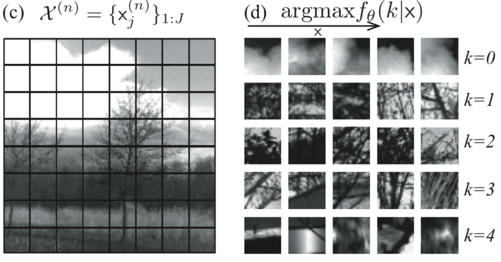
An interesting numerical experiment that highlights the RPM in action is in Figure 2 of the paper, two panels of which are shown below.

The $\xx_j$ are the pixel values of $J$ non-overlapping image patches, as shown in panel C below. These will certainly not be marginally independent. For example, the pixel values in two adjacent patches $\xx_1$ and $\xx_2$ at the top of the figure will tend to be correlated because both will be capturing the sky, clouds, etc. so $$p(\xx_1, \xx_2) \neq p(\xx_1) p(\xx_2).$$
However, we can introduce a latent variable for each patch that could indicate what type it is. Conditioned on these latent variables (labels), the pixel values will be much more independent. That is $$ p(\xx_1, \xx_2 | z_1, z_2) \approx p(\xx_1 | z_1) p(\xx_2 | z_2).$$ The panel on the right shows the patches with highest likelihood for each label, revealing that the RPM has found texture labels for each patch, conditioned on which the pixel values in different patches are independent.
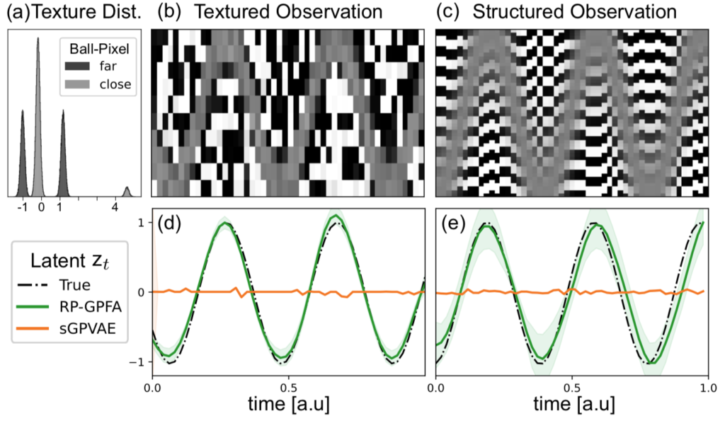
A second set of experiments demonstrates two limitations when using generative models. The observations in these experiments model a ball moving sinusoidally against a background.

In the first experiment, shown in panel B above, the pixel colours are determined by their proximity to the moving target. When pixels are far away, colours are chosen with equal probability from two identical Gaussians, one centred on +1, the other on -1 (the ‘far’ data in panel A). Colors are selected independently at each time step, which gives the far pixels their salt-and-pepper texture. The near pixels are also coloured by selecting from two Gaussians, but in this case, one of the Gaussians is much more likely to be selected than the other. This gives the pixels near the target a gray hue.
Crucially, the parameters of the Gaussians are chosen so that individual pixels in both conditions have the same mean and variance. The RPM is tested against a VAE model with a Gaussian Process prior on its latents to allow it to describe temporally varying latents. Because the means and variances of all pixels are the same, regardless of the position of the latent, the VAE doesn’t ‘see’ any variability to explain, and its estimate of the target’s position remains at zero (the orange curve in panel D). In other words, the generative model that the VAE uses to reproduce the observations and update its recognition model is blind to the higher-order correlations present in the observations that indicate the location of the target. It therefore sees nothing to explain and keeps its latent estimate at zero.
Summary
Many latent variable models used in unsupervised learning train the mapping of observations to latents by having the latents reconstruct the observations via a generative model. While this can sometimes be appropriate, it can be computationally wasteful when full reconstruction is not required, and problematic due to the biases caused by mismatched generative models. The Recognition Parameterized Model avoids these issues by not using a generative model at all. Instead, it looks for latents conditioned on which the observations become independent. Using this assumption, it formulates the joint distribution of the latents and observations in terms of recognition terms alone and allows the resulting functions to be arbitrarily parameterized (under some mild constraints), hence the name of the model. The resulting parameters of the model can be fitted using expectation maximization and this is a substantial part of the paper which I haven’t gone through in detail.
Leave a Reply